
CLIP, SigLIP & BLIP
These three lines of work produced the components almost every model in the comparison table is built from. CLIP established that language is a usable supervision signal for vision; SigLIP fixed the objective's engineering; BLIP attacked the data problem and then the connector problem. This page derives each objective, states precisely what it does and does not learn, and is explicit about the failure that all of them inherit.
Symbols used on this page are defined in the Nomenclature → learning.
1 · CLIP
1.1 The idea
Supervised vision needs labels, and labels bound you to a fixed vocabulary. CLIP's move was to train on 400 million image–text pairs scraped from the web with no manual labelling, using a task that needs no labels: given a batch of images and a batch of captions, match them up.
Two encoders map into a shared $d$-dimensional space, and both outputs are $L^2$-normalised so that the inner product is a cosine:
$$ \mathbf u_i = \frac{f_{\text{img}}(\mathbf x_i)}{\|f_{\text{img}}(\mathbf x_i)\|}, \qquad \mathbf v_j = \frac{f_{\text{txt}}(\mathbf t_j)}{\|f_{\text{txt}}(\mathbf t_j)\|}, \qquad s_{ij} = \mathbf u_i^{\mathsf T}\mathbf v_j \in [-1, 1] $$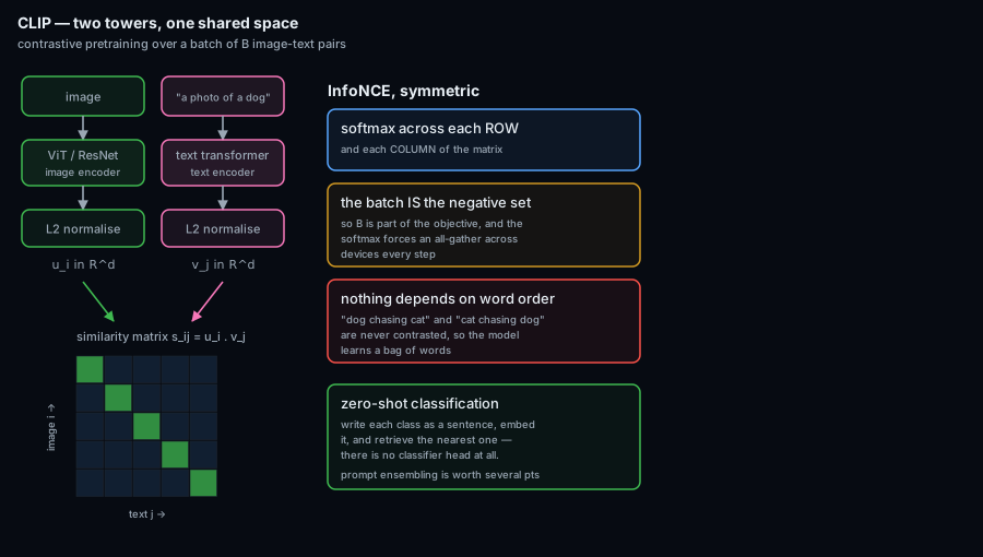
1.2 The InfoNCE objective, derived
In a batch of $B$ pairs, treat matching as $B$-way classification — twice, once in each direction. For the image-to-text direction, the probability that image $i$ matches caption $j$ is a softmax over the row of the similarity matrix, scaled by a temperature $\tau$:
$$ p(j \mid i) = \frac{\exp(s_{ij}/\tau)}{\sum_{k=1}^{B}\exp(s_{ik}/\tau)} $$The loss is the symmetric cross-entropy against the identity assignment:
$$ \mathcal L_{\text{CLIP}} = -\frac{1}{2B}\sum_{i=1}^{B}\Big[ \log p(i \mid i)_{\text{img}\to\text{txt}} + \log p(i \mid i)_{\text{txt}\to\text{img}}\Big] $$In code this is strikingly short, which is part of why it spread so fast:
logits = (img_emb @ txt_emb.T) * logit_scale.exp()   # (B, B)
labels = torch.arange(B, device=logits.device)
loss   = 0.5 * (F.cross_entropy(logits, labels)
              + F.cross_entropy(logits.T, labels))
1.3 The learned temperature, and why it is stored as a log
$\tau$ controls how sharply the model is required to discriminate. It is learned, not fixed, and it is parameterised as $\log(1/\tau)$ — a "logit scale" — for two reasons: the parameterisation keeps $\tau > 0$ automatically, and it makes the optimisation well-conditioned, since the useful range spans orders of magnitude.
| Regime | Effect on the loss | Consequence |
|---|---|---|
| $\tau$ large (soft) | Logits flattened; all pairs look similar | Weak gradient; the model under-discriminates |
| $\tau$ small (sharp) | Loss dominated by the single hardest negative | Sensitive to label noise — and web data is very noisy |
| Learned, then clipped | Converges to roughly 0.01 | CLIP clamps the logit scale at 100 because unconstrained training drove it there and destabilised |
1.4 Zero-shot classification as retrieval
CLIP has no classifier head. Classification is performed by writing the classes as sentences and retrieving the nearest one:
$$ \hat y = \arg\max_{c \in \mathcal C}\; \mathbf u^{\mathsf T}\, \mathbf v_c, \qquad \mathbf v_c = \text{normalise}\!\left(\frac{1}{|T|}\sum_{t \in T} f_{\text{txt}}\big(t(c)\big)\right) $$where $T$ is a set of prompt templates — "a photo of a {}", "a blurry photo of a {}", and so on — whose embeddings are averaged into one class vector. This prompt ensembling is worth several points of accuracy, which is an early instance of a theme that recurs throughout this section: a meaningful fraction of reported capability lives in the prompt rather than the weights. See VQA §3 for the same effect, less benignly.
1.5 The failure: a bag of words
Look again at the loss. The gradient pushes matched pairs together and mismatched pairs apart — and nothing else. Consider the caption "a dog chasing a cat". For the model to be penalised for confusing it with "a cat chasing a dog", the batch would have to contain the reversed caption paired with a different image. In a random batch drawn from web data, it essentially never does.
1.6 Batch size is part of the objective
The denominator in the softmax is the batch. The batch is the negative set, so batch size is not merely a throughput knob — it sets the difficulty of the task. CLIP trained at $B = 32{,}768$, which requires sharding across many devices and then an all-gather of every embedding so each device can compute a full row of the similarity matrix.
$$ \text{memory for logits} = O(B^2), \qquad \text{communication per step} = O(B \cdot d) $$This is the engineering burden SigLIP removes.
2 · SigLIP
2.1 The pairwise sigmoid objective
Replace one $B$-way classification with $B^2$ independent binary ones. Every cell of the similarity matrix is asked a yes/no question: is this pair matched?
$$ \mathcal L_{\text{SigLIP}} = \frac{1}{B}\sum_{i=1}^{B}\sum_{j=1}^{B} \log\!\Big(1 + \exp\big(z_{ij}(-t\,s_{ij} + b)\big)\Big), \qquad z_{ij} = \begin{cases}+1 & i=j\\ -1 & i\neq j\end{cases} $$This is just the logistic loss, $\log(1 + e^{-z\cdot\text{logit}})$, with logit $= t\,s_{ij} - b$. Two learned scalars: $t$ a temperature as before, and $b$ a bias.
2.2 Why the bias term is necessary, not cosmetic
The pair matrix is extremely imbalanced: $B$ positives against $B^2 - B$ negatives. At $B = 16{,}384$ that is one positive per 16,383 negatives. Initialised at $b = 0$, every pair starts at probability $\tfrac12$, so the loss is dominated by the enormous negative mass and the model's fastest descent direction is to call everything a non-match — which collapses the embedding.
Initialising $b$ strongly negative encodes the correct prior ("pairs are almost never matched"), so gradients from the rare positives are not drowned. This is the same reasoning as the prior-probability initialisation in focal loss for dense detection.
2.3 The comparison, and the result that mattered
| InfoNCE (CLIP) | Sigmoid (SigLIP) | |
|---|---|---|
| Normalisation | Softmax over the full batch | None — each pair independent |
| Needs all-gather | Yes | No — compute local chunks and sum |
| Logit memory | $O(B^2)$ materialised | $O(B^2)$ but chunkable |
| Small batches | Degrades badly | Works — usable at a few thousand |
| Very large batches | Keeps helping | Saturates ~32K |
| Extra parameters | $\tau$ | $t$ and $b$ |
SigLIP 2 extends the same objective with multilingual data, captioning and self-distillation objectives alongside the contrastive term, and variable-resolution variants — but the loss is unchanged.
3 · The BLIP family
BLIP's contributions are best understood as two separate attacks on two separate problems: BLIP-1 on data quality, BLIP-2 on connecting frozen models.
3.1 BLIP-1 — the captioner–filter bootstrap
Web alt-text is noisy: much of it is SEO keywords, filenames or boilerplate that describes nothing in the image. CLIP's answer was to drown the noise in scale. BLIP's answer was to clean the data using the model being trained:
The synthetic captions frequently describe the image better than the human alt-text did, and retraining on the filtered mixture improves results measurably. This is the direct ancestor of the recaptioning strategies that later drove DALL·E 3 and several models in the table — the lineage is why "better captions" is now considered as strong a lever as "more data".
BLIP-1's architecture, the MED (multimodal mixture of encoder–decoder), shares one parameter set across three roles selected by attention masking, trained with three losses at once:
| Mode | Loss | Purpose |
|---|---|---|
| Unimodal encoder | ITC — image-text contrastive | Align the two spaces, as in CLIP |
| Image-grounded encoder | ITM — image-text matching, binary | A fusion classifier; catches hard negatives the cosine misses |
| Image-grounded decoder | LM — captioning | Generation, which is what makes the captioner possible |
3.2 BLIP-2 — the Q-Former
By 2023 there were excellent frozen vision encoders and excellent frozen LLMs, and training either from scratch was wasteful. BLIP-2's question was how to connect them while training as little as possible. Its answer, the Q-Former, is a small transformer holding $k = 32$ learned query vectors:
Stage one trains the Q-Former against the frozen image encoder with BLIP-1's three objectives, each using a different attention mask over the queries and text. Stage two connects it to the frozen LLM and trains only on language modelling. The result is a fixed 32-token visual representation, independent of input resolution.
4 · What each contributed, in one table
| Model | Problem it attacked | Mechanism | Still used? |
|---|---|---|---|
| CLIP | Labels bound you to a fixed vocabulary | Contrastive training on 400M web pairs; zero-shot via prompts | Yes — vision towers, text conditioning, CLIP score |
| ALIGN | Is careful curation necessary? | 1.8B minimally-filtered pairs | As a result, not a component: scale substitutes for curation |
| SigLIP | The global softmax is a distributed-systems burden | Pairwise sigmoid with a learned bias | Yes — the current default vision tower |
| BLIP-1 | Web captions are noisy | CapFilt — generate and filter captions with the model itself | As a practice: recaptioning is now standard |
| BLIP-2 | Connect frozen towers cheaply | Q-Former, 32 learned queries, two-stage training | Largely not — superseded by MLP connectors |
| CoCa | Contrastive and generative were separate models | One decoder, split into unimodal and multimodal halves | As an idea — unified models are the current direction |
5 · SOTA comparison — contrastive encoders
Zero-shot ImageNet top-1 is the standard yardstick for this family, because it requires no fine-tuning and therefore measures the representation itself. The caveat from the model table applies in full: these are author-reported figures under differing protocols, so read tiers, not ranks.
| Model | Backbone | Res | Training pairs | IN-1k 0-shot | Objective | Open data? |
|---|---|---|---|---|---|---|
| CLIP | ViT-B/32 | 224 | 400M (WIT) | ~63% | InfoNCE | No |
| CLIP | ViT-L/14 | 336 | 400M (WIT) | ~76% | InfoNCE | No |
| ALIGN | EfficientNet-L2 | 289 | 1.8B noisy | ~76% | InfoNCE | No |
| OpenCLIP | ViT-H/14 | 224 | LAION-2B | ~78% | InfoNCE | Yes |
| OpenCLIP | ViT-G/14 | 224 | LAION-2B | ~80% | InfoNCE | Yes |
| EVA-CLIP | EVA ViT-g | 224 | ~2B merged | ~82% | InfoNCE, MIM init | Mostly |
| CoCa | ViT-g | 288 | JFT-3B + ALIGN | ~86%† | Contrastive + caption | No |
| SigLIP | So400m/14 | 384 | WebLI ~10B | ~83% | Pairwise sigmoid | No |
| SigLIP 2 | So400m | 384+ | WebLI, multilingual | ~85% | Sigmoid + caption + distil | No |
† CoCa's usually-quoted 86% is fine-tuned, not zero-shot, so it does not belong in this column at all. It is included precisely because it is the number normally cited for that model — exactly the apples-to-oranges comparison this section warns about.
5.1 Where the ranking changes
Zero-shot classification is one task. On the probes that isolate specific abilities, the ordering is not the same — which is the practical argument against choosing an encoder on IN-1k alone.
| Probe | What it measures | How this family does |
|---|---|---|
| COCO / Flickr retrieval | Image–text matching in both directions | Tracks IN-1k closely — same objective, same skill |
| Winoground | Word order and relational structure | At or below chance at group level, across the whole family, regardless of scale (§1.5) |
| ARO | Attribution, relation, order | Near-chance on relation and order subsets; scale does not rescue it |
| MMVP pairs | Visually distinct images with near-identical embeddings | Collapses pairs that a self-supervised encoder such as DINOv2 separates |
| Fine-grained (CUB, Cars) | Subordinate categories | Weaker than supervised baselines; the caption distribution simply lacks the vocabulary |
| OCR / text-in-image | Reading | Bounded by resolution, so a 384 px tower beats a larger 224 px one |
6 · Using them in practice
| Task | Use | Caution |
|---|---|---|
| Retrieval / embedding index | SigLIP 2, or OpenCLIP ViT-G | Normalise before indexing; cosine only means anything on the unit sphere |
| Zero-shot classification | Any CLIP-family model with prompt ensembling | Report the template set — it is worth several points |
| Scoring generated images | CLIP score, directional CLIP | Gameable: see editing §8 |
| Vision tower for a VLM | SigLIP-So400m or CLIP ViT-L/14-336 | Resolution is the ceiling on text-in-image — choose it first |
| Anything relational or compositional | — | Do not rely on a contrastive model. Word-order blindness is in the objective (§1.5) |
| Open-vocabulary detection | The alignment idea, per region | See GroundingDINO |
7 · References
The figures on this page are original redrawings in the site's palette, not reproductions — the architectures are credited to the papers below. Where a blog post is the clearest explanation of something, it is cited as such.
7.1 Primary sources
- Radford et al., Learning Transferable Visual Models From Natural Language Supervision (CLIP, ICML 2021).
- Jia et al., Scaling Up Visual and Vision-Language Representation Learning With Noisy Text Supervision (ALIGN, ICML 2021).
- Zhai et al., Sigmoid Loss for Language Image Pre-Training (SigLIP, ICCV 2023).
- Li et al., BLIP (ICML 2022) and BLIP-2 (ICML 2023).
- Yu et al., CoCa: Contrastive Captioners are Image-Text Foundation Models (2022).
- Cherti et al., Reproducible scaling laws for contrastive language-image learning (OpenCLIP, CVPR 2023).
- Sun et al., EVA-CLIP (2023).
7.2 On the bag-of-words failure
- Thrush et al., Winoground (CVPR 2022).
- Yuksekgonul et al., When and why vision-language models behave like bags-of-words, and what to do about it? (ICLR 2023).
- Tong et al., Eyes Wide Shut? Exploring the Visual Shortcomings of Multimodal LLMs (MMVP, CVPR 2024).
7.3 Useful secondary explanations
- Oord et al., Representation Learning with Contrastive Predictive Coding (InfoNCE, 2018) — the origin of the loss CLIP uses.
- Lin et al., Focal Loss for Dense Object Detection (ICCV 2017) — the prior-initialisation argument that explains SigLIP's bias term.
Related: Architecture modules · Model comparison table · Stable Diffusion deep dive · Visual question answering · Open problems · DINOv2 (vision without language)