
SurroundOcc — 2D→3D cross-attention
A detector answers “where are the cars?”. An occupancy network answers “what is in this cubic half-metre?” — for all 640,000 cubes around the ego, including the debris, overhangs and construction barriers that have no box class. SurroundOcc does this from six cameras and no LiDAR, by making the 3D grid the query and letting every voxel reach into whichever images can see it. This page derives that mechanism and reports every tensor shape from a run on this machine.
Symbols used here are collected in the Nomenclature.
Prerequisites: deformable attention (equation 8 there is the kernel used here), attention and FPN.
Read this before believing any colour in the videos below. The published SurroundOcc
checkpoint was unobtainable when this page was written — seven download routes, all dead
(Tsinghua Cloud, Weiyun, two GitHub release paths, and three Hugging Face mirrors). The model
below is built from the correct config and initialised from the
r101_dcn_fcos3d_pretrain backbone, which contains no
pts_bbox_head weights. So:
- Meaningful (measured here): tensor shapes, parameter counts, latency, throughput, peak GPU memory, the attention geometry, per-camera visibility counts.
- Meaningless: the predicted class of any voxel.
- Refused: mIoU. The inference script will not compute it without a head checkpoint, and the numbers in §8 are the paper's, clearly labelled as such.
The videos therefore show ground-truth occupancy (the released nuScenes-Occupancy
labels) over the real camera frames, and every single frame is stamped
GROUND TRUTH in the banner so a screenshot cannot be mistaken for a prediction.
1 · The output: what is actually predicted
Read from the config that ran (projects/configs/surroundocc/surroundocc.py), not from
the paper figure. The volume around the ego is
so the voxel is cubic at $v_x = (50-(-50))/200 = 0.5\,\text{m}$, and likewise $v_y = 0.5\,\text{m}$, $v_z = (3.0-(-5.0))/16 = 0.5\,\text{m}$:
$$ \underbrace{200 \times 200 \times 16}_{640{,}000 \text{ voxels}} \times (0.5\,\text{m})^3 \;=\; 100 \times 100 \times 8\ \text{m}^3 $$Correction to the figures elsewhere on this site. The perception deep dive describes an occupancy config with range $[-40,-40,-1,\,40,40,5.4]$ at $0.4\,\text{m}$ and calls it “camera-first and LSS-based”. That describes a different (LSS-style) occupancy head. The actual SurroundOcc released by Wei et al. uses the range and resolution above, and its 2D→3D step is spatial cross-attention, not Lift-Splat-Shoot: there is no depth distribution and no splat. The distinction is the whole subject of §4.
Each voxel carries one of $C = 17$ labels: index 0 is empty, and 1–16 are the nuScenes semantic classes, in exactly this order:
| 1–5 | 6–10 | 11–16 |
|---|---|---|
| barrier, bicycle, bus, car, construction_vehicle | motorcycle, pedestrian, traffic_cone, trailer, truck | driveable_surface, other_flat, sidewalk, terrain, manmade, vegetation |
Class 0 is not a “background” class to be ignored — it is the single most common label, and §6 explains why the loss has to be built around that imbalance.
2 · What it looks like, over real scenes
320 frames rendered at 3840×2160 from eight nuScenes validation scenes, selected by a condition-stratified sampler over the 150 real val scenes (§7): 2 night, 2 rain, 4 day, spanning all four recording locations. Each frame shows the six camera images, the BEV projection (topmost occupied voxel per column), a 3D view, and a per-class occupied-voxel histogram.
yuv420p with
+faststart so they stream and decode in Safari. A 3840×2160 master
(112 MB) exists outside the deployed tree and is not shipped to visitors.
The histogram panel is the useful part for debugging: on a typical frame it reads
manmade and vegetation around $10^4$ voxels, car around
600, and traffic_cone in the single digits — a span of four orders of
magnitude, which is why it is drawn on a symlog axis and why §6's loss needs the
class-balancing terms.
3 · The forward pass, with measured shapes
All shapes below were captured with forward hooks during a real
simple_test call on an RTX 6000 Ada (sm_89), batch size $B=1$, six cameras.
The probe (scripts/probe_architecture.py) registers 697 hooks and writes
arch_probe.json; the diagram, the tensor table in §3.6 and every number in this
section are read from that file, and the maths is read from the forward passes in
projects/mmdet3d_plugin/surroundocc/. Where the code and the paper disagree, this page
follows the code and says so.
3.1 The diagram
Interactive: scroll, zoom and pan. Image tensor at the top, logits and losses at the bottom right.
The three columns are the three scales; the dashed pink frame is the per-scale
OccEncoder, the dashed blue frame the image encoder. Every edge is labelled with the
tensor it carries.
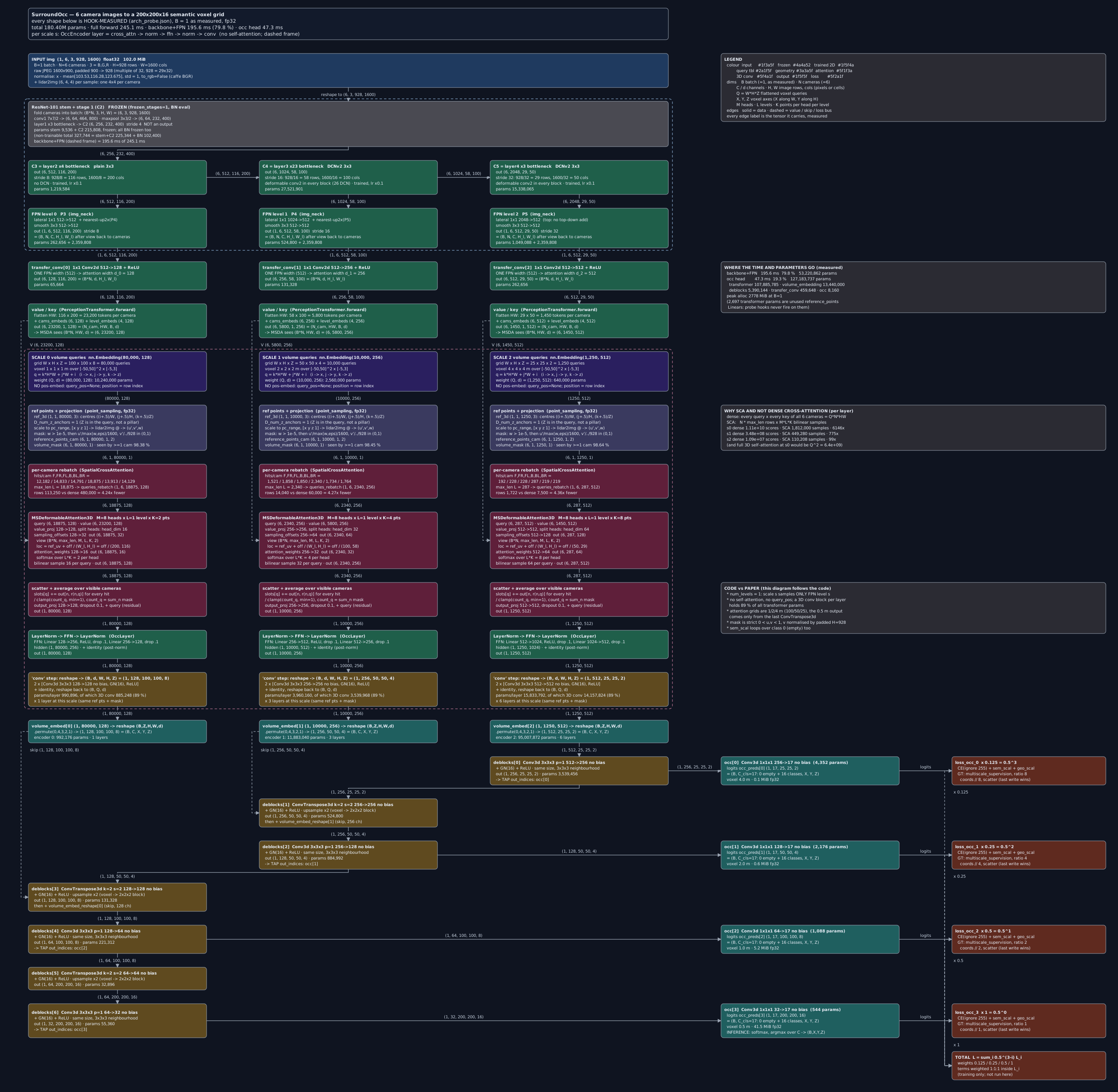
Downloads. draw.io source (editable — open at app.diagrams.net) · SVG (vector, scales to any size)
Regenerate both with
python scripts/gen_drawio.py /mnt/mydata/surroundocc_runs/arch_probe.json --outdir <site>/deeplearning/figs/surroundocc --table-html tensors.html
from the surroundocc/ repo. The generator reads only the probe JSON, asserts it against
the config arithmetic (e.g. that the three embedding tables sum to the measured
volume_embedding count, and that every FPN level is exactly $H/2^{\ell+3}$), and refuses
to write if any box is too small for its text, any two boxes overlap, any edge is unlabelled, any
label sits on a box or any edge runs underneath an unrelated box. It also emits the tensor table
of §3.6, so the table and the picture come from the same parse.
3.2 Images to multi-scale features
The six $1600 \times 900$ JPEGs are normalised with caffe-style BGR statistics ($\mu = [103.530, 116.280, 123.675]$, $\sigma = 1$, no RGB swap) and padded to a multiple of 32, giving $928 \times 1600$. They enter as one tensor with the camera axis folded in:
$$ \mathbf{I} \in \mathbb{R}^{B \times N \times 3 \times H \times W} = \mathbb{R}^{1 \times 6 \times 3 \times 928 \times 1600}, \qquad H = 32\left\lceil \tfrac{900}{32} \right\rceil = 32 \cdot 29 = 928 \tag{1} $$
with dimensions batch, camera, colour (B,G,R order, since to_rgb=False), row, column.
The detector folds the camera axis into the batch, $(BN, 3, H, W) = (6, 3, 928, 1600)$, so the
backbone sees six independent images. GridMask is a no-op at inference
(not self.training). ResNet-101 (caffe style) has a stride-4 stem
(7×7/2 conv, 3×3/2 max-pool) and four stages, each but the first halving resolution.
With out_indices=(1,2,3) the outputs are C3, C4, C5, not C2, and FPN level
$\ell \in \{0,1,2\}$ sits at stride $2^{\ell+3}$:
where $\tilde P_{\ell+1}$ is the pre-smoothing lateral sum one level up (absent at the top) and
every $P_\ell$ has 512 channels. Padding to 928 is what makes all three divisions exact: 900 is
not divisible by 8, so without it the stride-8 map would not tile the image. Stage C2 and the stem
are frozen (frozen_stages=1), every BatchNorm is frozen (norm_eval=True),
stages 3 and 4 use DCNv2 for every 3×3 (26 deformable convs), and the trainable backbone
runs at $0.1\times$ the head's learning rate. Measured, with the camera axis restored:
| level | shape $(B, N_{\text{cam}}, C, H_\ell, W_\ell)$ | stride | tokens per camera |
|---|---|---|---|
| 0 | $(1, 6, 512, 116, 200)$ | 8 | 23,200 |
| 1 | $(1, 6, 512, 58, 100)$ | 16 | 5,800 |
| 2 | $(1, 6, 512, 29, 50)$ | 32 | 1,450 |
A $1\times1$ transfer_conv (with bias, then ReLU) maps the single FPN width to the
attention width each 3D scale uses, so there is one FPN width and three attention widths:
Scale $s$ therefore pairs with exactly one FPN level, the one with the same index: the finest image map (stride 8) feeds the finest voxel grid, the coarsest image map feeds the coarsest grid. Flattened, with a learned camera embedding (6, $d_s$) and level embedding added, these become the attention values $(N, H_sW_s, B, d_s) = (6, 23200, 1, 128)$, $(6, 5800, 1, 256)$ and $(6, 1450, 1, 512)$.
3.3 The 3D queries and the voxel grids
This is the structural choice that defines the model. The queries are a learned embedding table indexed by 3D position — one vector per voxel, at three resolutions:
| scale $s$ | $(H_s, W_s, Z_s)$ | queries $= H_sW_sZ_s$ | $d_s$ | parameters |
|---|---|---|---|---|
| 0 | $(100, 100, 8)$ | 80,000 | 128 | 10,240,000 |
| 1 | $(50, 50, 4)$ | 10,000 | 256 | 2,560,000 |
| 2 | $(25, 25, 2)$ | 1,250 | 512 | 640,000 |
Those sum to exactly the measured volume_embedding parameter count, term by term
scale 0, 1, 2 (the generator asserts this before drawing):
Each scale tiles the same box $[-50,50]^2 \times [-5,3]$ m, so its voxel edge and the centre of voxel $(i,j,k)$, $0 \le i \lt W_s$, $0 \le j \lt H_s$, $0 \le k \lt Z_s$, are
$$ v_s = \frac{100}{W_s} = \frac{100}{H_s} = \frac{8}{Z_s} = 1,\ 2,\ 4\ \text{m}, \qquad \mathbf{c}_{ijk} = \Big(-50 + (i+\tfrac12)v_s,\; -50 + (j+\tfrac12)v_s,\; -5 + (k+\tfrac12)v_s\Big), \qquad q = k\,H_sW_s + j\,W_s + i \tag{5} $$
where $q$ is the row of the embedding table, i.e. the flattening order the code uses
(get_reference_points builds a $(Z,H,W)$ lattice and flattens it). The attention
grids are therefore at 1, 2 and 4 m: the finest attended grid, $(100,100,8)$, is half the
output resolution in each axis, and the 0.5 m output only appears after the last transposed
convolution in §3.5. The network never attends at full resolution. There is also no
positional embedding: query_pos is None everywhere, so a query knows
where it is only through (a) which row of the table it is, learned, and (b) where its reference
point projects, which is geometry.
3.4 One encoder layer, as the code runs it
Scale $s$ runs $L_s = 1, 3, 6$ OccLayers, so the coarsest grid gets the most depth.
The config's operation_order is
('cross_attn', 'norm', 'ffn', 'norm', 'conv'): a post-norm transformer layer with
no self-attention, followed by a 3D convolution block. For queries
$\mathbf{Z} \in \mathbb{R}^{B \times Q_s \times d_s}$:
$\mathrm{SCA}$ includes its own residual (§4.4), dropout is 0.1 in the FFN and SCA, and
$\mathcal{R}$ reshapes $(B, Q_s, d_s) \to (B, d_s, W_s, H_s, Z_s)$ with
reshape(B,Z,H,W,d).permute(0,4,3,2,1). The convolution block is not in the paper's
figure and is easy to miss, but it dominates the head: measured, the six 3D convs per scale-2
layer are $2 \times 512 \cdot 512 \cdot 27 = 14{,}155{,}776$ weights, and across all ten layers
the 3D convs hold 96.4 M of the 107.9 M transformer parameters (89 %). The
"transformer" is mostly a 3D CNN with a camera-sampling step in front.
3.5 The 3D deconvolution trunk and the four heads
The three encoded volumes $\mathbf{V}_s = \mathcal{R}(\mathbf{Z}^{(s)}) \in
\mathbb{R}^{B \times d_s \times W_s \times H_s \times Z_s}$ are fused coarse-to-fine by seven
deblocks, each a conv followed by GN(16) and ReLU. Even indices are
$3\times3\times3$, pad 1, stride 1 convs (size unchanged); odd indices are
ConvTranspose3d with kernel 2, stride 2, pad 0, whose output size is
so each one paints a $2\times2\times2$ block per input voxel with no overlap. The forward loop
adds a skip after deblocks 1 and 3 only (elif i < len(self.deblocks) - 2):
The four $1\times1\times1$ classifiers tap $\mathbf{h}_0, \mathbf{h}_2, \mathbf{h}_4, \mathbf{h}_6$
(out_indices=[0,2,4,6]), giving logits at voxel sizes 4, 2, 1 and 0.5 m:
| $i$ | occ_preds[i] shape | loss weight $0.5^{\,3-i}$ |
|---|---|---|
| 0 | $(1, 17, 25, 25, 2)$ | 0.125 |
| 1 | $(1, 17, 50, 50, 4)$ | 0.25 |
| 2 | $(1, 17, 100, 100, 8)$ | 0.5 |
| 3 | $(1, 17, 200, 200, 16)$ | 1.0 |
Only occ_preds[3] is used at inference:
$\hat y_{xyz} = \arg\max_c \operatorname{softmax}(\boldsymbol{\ell}_3)_{c,xyz}$
(generate_output), a $(1, 200, 200, 16)$ label volume. The videos on this page draw
ground truth instead, for the reasons in the callout at the top.
3.6 Every tensor, with its dimensions
Generated by gen_drawio.py --table-html from the same probe parse as the diagram.
Memory is the size of one materialised copy at $B=1$ (fp32, or 1 byte for the boolean mask), not
the allocator's peak. For repeated encoder layers the first layer is listed; later layers at the
same scale have identical shapes. Dimension names: $B$ batch, $N$ cameras, $d_s$ attention width
at scale $s$, $H_\ell, W_\ell$ FPN rows and columns, $Q_s = W_sH_sZ_s$ queries, $X,Y,Z$ voxel axes,
$M$ heads, $L$ levels, $K$ points.
| stage | tensor | shape | dimensions | dtype | memory, $B=1$ | code |
|---|---|---|---|---|---|---|
| input | img | (1, 6, 3, 928, 1600) | B, N_cam, BGR, H, W | float32 | 101.95 MiB | projects/mmdet3d_plugin/surroundocc/detectors/surroundocc.py:extract_img_feat |
| input | lidar2img | (1, 6, 4, 4) | B, N_cam, 4, 4 (ego->pixel) | float32 | 384 B | projects/mmdet3d_plugin/surroundocc/modules/encoder.py:point_sampling |
| backbone | conv1 out | (6, 64, 464, 800) | B*N, C, H/2, W/2 | float32 | 543.75 MiB | mmdet ResNet.forward |
| backbone | C2 (layer1) | (6, 256, 232, 400) | B*N, C, H/4, W/4 | float32 | 543.75 MiB | mmdet ResNet.forward |
| backbone | C3 (layer2) | (6, 512, 116, 200) | B*N, C, H/8, W/8 | float32 | 271.88 MiB | mmdet ResNet.forward (out_indices=(1, 2, 3)) |
| backbone | C4 (layer3) | (6, 1024, 58, 100) | B*N, C, H/16, W/16 | float32 | 135.94 MiB | mmdet ResNet.forward (out_indices=(1, 2, 3)) |
| backbone | C5 (layer4) | (6, 2048, 29, 50) | B*N, C, H/32, W/32 | float32 | 67.97 MiB | mmdet ResNet.forward (out_indices=(1, 2, 3)) |
| FPN | mlvl_feats[0] | (1, 6, 512, 116, 200) | B, N_cam, C, H/8, W/8 | float32 | 271.88 MiB | projects/mmdet3d_plugin/surroundocc/detectors/surroundocc.py:extract_img_feat |
| FPN | mlvl_feats[1] | (1, 6, 512, 58, 100) | B, N_cam, C, H/16, W/16 | float32 | 67.97 MiB | projects/mmdet3d_plugin/surroundocc/detectors/surroundocc.py:extract_img_feat |
| FPN | mlvl_feats[2] | (1, 6, 512, 29, 50) | B, N_cam, C, H/32, W/32 | float32 | 16.99 MiB | projects/mmdet3d_plugin/surroundocc/detectors/surroundocc.py:extract_img_feat |
| head | view_features[0] | (1, 6, 128, 116, 200) | B, N_cam, d_s, H_l, W_l | float32 | 67.97 MiB | projects/mmdet3d_plugin/surroundocc/dense_heads/occ_head.py:forward |
| head | view_features[1] | (1, 6, 256, 58, 100) | B, N_cam, d_s, H_l, W_l | float32 | 33.98 MiB | projects/mmdet3d_plugin/surroundocc/dense_heads/occ_head.py:forward |
| head | view_features[2] | (1, 6, 512, 29, 50) | B, N_cam, d_s, H_l, W_l | float32 | 16.99 MiB | projects/mmdet3d_plugin/surroundocc/dense_heads/occ_head.py:forward |
| encoder | value[0] | (6, 23200, 1, 128) | N_cam, HW_l, B, d_s | float32 | 67.97 MiB | projects/mmdet3d_plugin/surroundocc/modules/transformer.py:forward |
| encoder | value[1] | (6, 5800, 1, 256) | N_cam, HW_l, B, d_s | float32 | 33.98 MiB | projects/mmdet3d_plugin/surroundocc/modules/transformer.py:forward |
| encoder | value[2] | (6, 1450, 1, 512) | N_cam, HW_l, B, d_s | float32 | 16.99 MiB | projects/mmdet3d_plugin/surroundocc/modules/transformer.py:forward |
| encoder | volume_queries[0] | (80000, 128) | Q_s = W*H*Z flattened (k,j,i), d_s | float32 | 39.06 MiB | projects/mmdet3d_plugin/surroundocc/dense_heads/occ_head.py:forward (volume_embedding.weight) |
| encoder | ref_3d[0] | (1, 1, 80000, 3) | B, D=1, Q_s, xyz in (0,1) | float32 | 0.92 MiB | projects/mmdet3d_plugin/surroundocc/modules/encoder.py:get_reference_points |
| encoder | reference_points_cam[0] | (6, 1, 80000, 1, 2) | N_cam, B, Q_s, D=1, uv in (0,1) | float32 | 3.66 MiB | projects/mmdet3d_plugin/surroundocc/modules/encoder.py:point_sampling |
| encoder | volume_mask[0] | (6, 1, 80000, 1) | N_cam, B, Q_s, D=1 | bool | 0.46 MiB | projects/mmdet3d_plugin/surroundocc/modules/encoder.py:point_sampling |
| encoder | queries_rebatch[0] | (1, 6, 18875, 128) | B, N_cam, max_len, d_s | float32 | 55.30 MiB | projects/mmdet3d_plugin/surroundocc/modules/spatial_cross_attention.py:SpatialCrossAttention.forward |
| encoder | sampling_offsets[0] | (6, 18875, 8, 1, 2, 2) | B*N, max_len, M, L, K, xy | float32 | 13.82 MiB | projects/mmdet3d_plugin/surroundocc/modules/spatial_cross_attention.py:MSDeformableAttention3D.forward |
| encoder | attention_weights[0] | (6, 18875, 8, 1, 2) | B*N, max_len, M, L, K (softmax over L*K) | float32 | 6.91 MiB | projects/mmdet3d_plugin/surroundocc/modules/spatial_cross_attention.py:MSDeformableAttention3D.forward |
| encoder | msda_out[0] | (6, 18875, 128) | B*N, max_len, d_s | float32 | 55.30 MiB | projects/mmdet3d_plugin/surroundocc/modules/spatial_cross_attention.py:MSDeformableAttention3D.forward |
| encoder | sca_out[0] | (1, 80000, 128) | B, Q_s, d_s | float32 | 39.06 MiB | projects/mmdet3d_plugin/surroundocc/modules/spatial_cross_attention.py:SpatialCrossAttention.forward |
| encoder | ffn_hidden[0] | (1, 80000, 256) | B, Q_s, F_s | float32 | 78.12 MiB | mmcv FFN.forward |
| encoder | conv_in[0] | (1, 128, 100, 100, 8) | B, d_s, X=W, Y=H, Z | float32 | 39.06 MiB | projects/mmdet3d_plugin/surroundocc/modules/encoder.py:OccLayer.forward |
| head | volume_embed_reshape[0] | (1, 128, 100, 100, 8) | B, d_s, X, Y, Z | float32 | 39.06 MiB | projects/mmdet3d_plugin/surroundocc/dense_heads/occ_head.py:forward |
| encoder | volume_queries[1] | (10000, 256) | Q_s = W*H*Z flattened (k,j,i), d_s | float32 | 9.77 MiB | projects/mmdet3d_plugin/surroundocc/dense_heads/occ_head.py:forward (volume_embedding.weight) |
| encoder | ref_3d[1] | (1, 1, 10000, 3) | B, D=1, Q_s, xyz in (0,1) | float32 | 0.11 MiB | projects/mmdet3d_plugin/surroundocc/modules/encoder.py:get_reference_points |
| encoder | reference_points_cam[1] | (6, 1, 10000, 1, 2) | N_cam, B, Q_s, D=1, uv in (0,1) | float32 | 0.46 MiB | projects/mmdet3d_plugin/surroundocc/modules/encoder.py:point_sampling |
| encoder | volume_mask[1] | (6, 1, 10000, 1) | N_cam, B, Q_s, D=1 | bool | 0.06 MiB | projects/mmdet3d_plugin/surroundocc/modules/encoder.py:point_sampling |
| encoder | queries_rebatch[1] | (1, 6, 2340, 256) | B, N_cam, max_len, d_s | float32 | 13.71 MiB | projects/mmdet3d_plugin/surroundocc/modules/spatial_cross_attention.py:SpatialCrossAttention.forward |
| encoder | sampling_offsets[1] | (6, 2340, 8, 1, 4, 2) | B*N, max_len, M, L, K, xy | float32 | 3.43 MiB | projects/mmdet3d_plugin/surroundocc/modules/spatial_cross_attention.py:MSDeformableAttention3D.forward |
| encoder | attention_weights[1] | (6, 2340, 8, 1, 4) | B*N, max_len, M, L, K (softmax over L*K) | float32 | 1.71 MiB | projects/mmdet3d_plugin/surroundocc/modules/spatial_cross_attention.py:MSDeformableAttention3D.forward |
| encoder | msda_out[1] | (6, 2340, 256) | B*N, max_len, d_s | float32 | 13.71 MiB | projects/mmdet3d_plugin/surroundocc/modules/spatial_cross_attention.py:MSDeformableAttention3D.forward |
| encoder | sca_out[1] | (1, 10000, 256) | B, Q_s, d_s | float32 | 9.77 MiB | projects/mmdet3d_plugin/surroundocc/modules/spatial_cross_attention.py:SpatialCrossAttention.forward |
| encoder | ffn_hidden[1] | (1, 10000, 512) | B, Q_s, F_s | float32 | 19.53 MiB | mmcv FFN.forward |
| encoder | conv_in[1] | (1, 256, 50, 50, 4) | B, d_s, X=W, Y=H, Z | float32 | 9.77 MiB | projects/mmdet3d_plugin/surroundocc/modules/encoder.py:OccLayer.forward |
| head | volume_embed_reshape[1] | (1, 256, 50, 50, 4) | B, d_s, X, Y, Z | float32 | 9.77 MiB | projects/mmdet3d_plugin/surroundocc/dense_heads/occ_head.py:forward |
| encoder | volume_queries[2] | (1250, 512) | Q_s = W*H*Z flattened (k,j,i), d_s | float32 | 2.44 MiB | projects/mmdet3d_plugin/surroundocc/dense_heads/occ_head.py:forward (volume_embedding.weight) |
| encoder | ref_3d[2] | (1, 1, 1250, 3) | B, D=1, Q_s, xyz in (0,1) | float32 | 15,000 B | projects/mmdet3d_plugin/surroundocc/modules/encoder.py:get_reference_points |
| encoder | reference_points_cam[2] | (6, 1, 1250, 1, 2) | N_cam, B, Q_s, D=1, uv in (0,1) | float32 | 0.06 MiB | projects/mmdet3d_plugin/surroundocc/modules/encoder.py:point_sampling |
| encoder | volume_mask[2] | (6, 1, 1250, 1) | N_cam, B, Q_s, D=1 | bool | 7,500 B | projects/mmdet3d_plugin/surroundocc/modules/encoder.py:point_sampling |
| encoder | queries_rebatch[2] | (1, 6, 287, 512) | B, N_cam, max_len, d_s | float32 | 3.36 MiB | projects/mmdet3d_plugin/surroundocc/modules/spatial_cross_attention.py:SpatialCrossAttention.forward |
| encoder | sampling_offsets[2] | (6, 287, 8, 1, 8, 2) | B*N, max_len, M, L, K, xy | float32 | 0.84 MiB | projects/mmdet3d_plugin/surroundocc/modules/spatial_cross_attention.py:MSDeformableAttention3D.forward |
| encoder | attention_weights[2] | (6, 287, 8, 1, 8) | B*N, max_len, M, L, K (softmax over L*K) | float32 | 0.42 MiB | projects/mmdet3d_plugin/surroundocc/modules/spatial_cross_attention.py:MSDeformableAttention3D.forward |
| encoder | msda_out[2] | (6, 287, 512) | B*N, max_len, d_s | float32 | 3.36 MiB | projects/mmdet3d_plugin/surroundocc/modules/spatial_cross_attention.py:MSDeformableAttention3D.forward |
| encoder | sca_out[2] | (1, 1250, 512) | B, Q_s, d_s | float32 | 2.44 MiB | projects/mmdet3d_plugin/surroundocc/modules/spatial_cross_attention.py:SpatialCrossAttention.forward |
| encoder | ffn_hidden[2] | (1, 1250, 1024) | B, Q_s, F_s | float32 | 4.88 MiB | mmcv FFN.forward |
| encoder | conv_in[2] | (1, 512, 25, 25, 2) | B, d_s, X=W, Y=H, Z | float32 | 2.44 MiB | projects/mmdet3d_plugin/surroundocc/modules/encoder.py:OccLayer.forward |
| head | volume_embed_reshape[2] | (1, 512, 25, 25, 2) | B, d_s, X, Y, Z | float32 | 2.44 MiB | projects/mmdet3d_plugin/surroundocc/dense_heads/occ_head.py:forward |
| trunk | deblocks[0] out | (1, 256, 25, 25, 2) | B, C, X, Y, Z | float32 | 1.22 MiB | projects/mmdet3d_plugin/surroundocc/dense_heads/occ_head.py:forward |
| trunk | deblocks[1] out | (1, 256, 50, 50, 4) | B, C, X, Y, Z | float32 | 9.77 MiB | projects/mmdet3d_plugin/surroundocc/dense_heads/occ_head.py:forward |
| trunk | deblocks[2] out | (1, 128, 50, 50, 4) | B, C, X, Y, Z | float32 | 4.88 MiB | projects/mmdet3d_plugin/surroundocc/dense_heads/occ_head.py:forward |
| trunk | deblocks[3] out | (1, 128, 100, 100, 8) | B, C, X, Y, Z | float32 | 39.06 MiB | projects/mmdet3d_plugin/surroundocc/dense_heads/occ_head.py:forward |
| trunk | deblocks[4] out | (1, 64, 100, 100, 8) | B, C, X, Y, Z | float32 | 19.53 MiB | projects/mmdet3d_plugin/surroundocc/dense_heads/occ_head.py:forward |
| trunk | deblocks[5] out | (1, 64, 200, 200, 16) | B, C, X, Y, Z | float32 | 156.25 MiB | projects/mmdet3d_plugin/surroundocc/dense_heads/occ_head.py:forward |
| trunk | deblocks[6] out | (1, 32, 200, 200, 16) | B, C, X, Y, Z | float32 | 78.12 MiB | projects/mmdet3d_plugin/surroundocc/dense_heads/occ_head.py:forward |
| output | occ_preds[0] | (1, 17, 25, 25, 2) | B, C_cls=17, X, Y, Z | float32 | 0.08 MiB | projects/mmdet3d_plugin/surroundocc/dense_heads/occ_head.py:forward |
| output | occ_preds[1] | (1, 17, 50, 50, 4) | B, C_cls=17, X, Y, Z | float32 | 0.65 MiB | projects/mmdet3d_plugin/surroundocc/dense_heads/occ_head.py:forward |
| output | occ_preds[2] | (1, 17, 100, 100, 8) | B, C_cls=17, X, Y, Z | float32 | 5.19 MiB | projects/mmdet3d_plugin/surroundocc/dense_heads/occ_head.py:forward |
| output | occ_preds[3] | (1, 17, 200, 200, 16) | B, C_cls=17, X, Y, Z | float32 | 41.50 MiB | projects/mmdet3d_plugin/surroundocc/dense_heads/occ_head.py:forward |
Code paths are relative to projects/mmdet3d_plugin/surroundocc/. Two rows are worth
reading twice: reference_points_cam[0] holds all $6 \times 80000$ projections even
though only 113,250 rows are ever attended, and occ_preds[3] at 41.5 MiB is the
largest activation in the head.
4 · Spatial cross-attention, derived
The name is backwards from the data flow, and it is worth being precise about this because it confuses people. Geometrically the mechanism runs 3D→2D: we take a known 3D point and project it into the images to find out where to look. Informationally it runs 2D→3D: image features flow into the voxel. There is no depth estimation anywhere.
4.1 From query index to metric point
Let a query at scale $s$ have integer grid index $(i,j,k)$, table row $q$ as in (5).
get_reference_points builds a normalised cell-centre lattice with
torch.linspace(0.5, W-0.5, W) / W (and likewise for $H$, $Z$), stacked as $(x,y,z)$
and flattened over $(Z,H,W)$, so ref_3d has shape $(B, D, Q_s, 3)$ with $D=1$:
point_sampling (forced to fp32) maps it into the ego/LiDAR frame by scaling to the
point-cloud range, with $\mathbf{r}_{\min} = (-50,-50,-5)$ and $\mathbf{r}_{\max} = (50,50,3)$,
which reproduces the voxel centre $\mathbf{c}_{ijk}$ of (5) exactly:
4.2 Project into every camera
For camera $n$ with projection $\mathbf{T}_n \in \mathbb{R}^{4\times4}$ (the
lidar2img matrix, built as viewpad @ lidar2cam.T), the code appends a 1,
broadcasts to $(D, B, N, Q_s, 4, 1)$ and does one batched matmul:
where $w_{nq}$ is depth along the optical axis, the fourth row is discarded, and $(W, H) = (1600,
928)$ is the padded img_shape, not the 900-row JPEG: the bottom 28 rows are
padding, so $\hat v$ of a real pixel never exceeds $900/928 = 0.970$. The mask is computed in two
steps, depth first and bounds after the divide, with strict inequalities:
followed by nan_to_num. The $\max(w,\epsilon)$ only keeps the divide finite for
points behind the camera; those are already rejected by the depth test, which is why it is
applied before the divide. Outputs: reference_points_cam $(N, B, Q_s, D, 2)$ and
volume_mask $(N, B, Q_s, D)$, measured $(6,1,80000,1,2)$ and $(6,1,80000,1)$ at
scale 0. This mask is the entire geometric content of the method. It is computed from calibration,
is not learned, and carries no uncertainty, which is why a wrong lidar2img silently
produces a plausible-looking but meaningless volume instead of an error.
The one number that separates this from BEVFormer. BEVFormer's spatial cross-attention gives each BEV query a pillar of $D$ height anchors ($D=4$ in the paper) and averages the samples over them. Measured here, at every one of the three scales:
$$ D_{\text{num\_z\_anchors}} = 1 $$
Because $Z$ is already part of the query index, each query is a single point, not a pillar.
The num_Z_anchors reshape inside the attention is an identity operation in this
configuration. Any BEVFormer figure showing a stack of anchors per query is wrong for this code.
4.3 Per-camera rebatching, and why
With 80,000 queries and 6 cameras, the dense approach would run attention on
$6 \times 80000 = 480{,}000$ query slots and throw away everything the mask rejects. Instead
SpatialCrossAttention.forward gathers, for each camera, the index set of queries that
hit it, pads to the largest such count, and runs one batched attention of shape
$(BN, L_{\max}, d_s)$:
and the same for the reference points. The padded rows are real work: they are sampled at
$(0,0)$ and their outputs discarded, so the batch costs $N L_{\max}$ rows, not
$\sum_n |\mathcal{V}_n|$. One quirk worth knowing: $\mathcal{V}_n$ is taken from
mask_per_img[0], the first sample in the batch, and reused for every sample. At
$B=1$, as measured here, that is exact.
Measured at scale 0 (80,000 queries, 1600×900 images, a real val frame):
| camera | queries hit | fraction of 80,000 |
|---|---|---|
| CAM_FRONT | 12,182 | 15.2% |
| CAM_FRONT_RIGHT | 14,833 | 18.5% |
| CAM_FRONT_LEFT | 14,791 | 18.5% |
| CAM_BACK | 18,875 | 23.6% |
| CAM_BACK_LEFT | 13,913 | 17.4% |
| CAM_BACK_RIGHT | 14,129 | 17.7% |
| union (seen by $\ge 1$ camera): 98.38% · $L = 18{,}875$ | ||
So the rebatching saves
$$ \frac{N\,Q_0}{N\,L_{\max}} = \frac{6 \times 80000}{6 \times 18875} = \frac{480000}{113250} \approx 4.24\times $$
in attention work. Two things in that table are worth pausing on. CAM_BACK wins
because it is the widest-FOV camera on the nuScenes rig, so it covers more of the grid than the
front camera does. And the union is 98.38%, not 100% — roughly 1,300 voxels of the 80,000
are in the grid but outside every frustum (directly above and below the vehicle, and in the
small blind wedges between adjacent FOVs). The same measurement at the coarser scales gives
$L_{\max} = 2340$ of 10,000 ($4.27\times$) and $287$ of 1,250 ($4.36\times$), with union coverage
98.45 % and 98.64 %.
4.4 Sample, scatter, normalise
Each gathered row runs MSDeformableAttention3D against its own camera's value map.
The config is $M = 8$ heads and, contrary to the "multi-scale" in the name, $L = 1$ level: scale
$s$ only ever samples FPN level $s$ (an earlier version of this page said three levels and 64
channels per head; the measured head widths are $d_s/M = 16, 32, 64$). With $K_s = 2, 4, 8$
points, row $r$ of camera $n$ carrying query $\mathbf{z}$ and reference $\hat{\mathbf{p}} =
(\hat u, \hat v)$ computes
where $\Vert$ concatenates the $M$ head outputs of width $d_s/M$ back to $d_s$ (this module has no
output projection of its own; it is applied after the camera average below), and the softmax runs
over the $L K_s$ entries of each head. Offsets are in pixels of level $l$: dividing by
$(W_l, H_l) = (200, 116)$ at scale 0 turns them into normalised image units. At initialisation the
offset weights are zero and the bias points head $m$ in direction $\theta_m = 2\pi m/M$ at radius
$k$ pixels for point $k$, so the eight heads start as a star of rays around the reference, and the
attention weights start uniform. $\mathcal{S}$ is bilinear sampling with zero padding in the
align_corners=False convention (CUDA kernel: h_im = loc_h * H - 0.5):
with $\mathbf{V}[b,a] = \mathbf{0}$ outside the map. Each row therefore reads
$M L K_s = 16, 32, 64$ bilinear samples at scales 0, 1, 2. The rows are then scattered back to
their query slots, summed over cameras and divided by the number of cameras that saw the voxel,
after which a shared output projection, dropout 0.1 and the residual are applied
(slots / count[..., None], count = clamp(..., min=1)):
The $\max(\cdot, 1)$ in the denominator is not cosmetic. For the ~1.6% of voxels no camera sees, the numerator is zero, so the attention term is $\mathbf{W}_o\mathbf{0} + \mathbf{b}_o$ and after the residual connection the voxel carries only its own learned query embedding plus a constant. (The 3D convolutions of (7) then mix in its neighbours, so it is not completely blind, but it has no image evidence of its own.) Those voxels are not “unknown” — they are filled in from the prior baked into the embedding table during training. That is a real limitation worth naming: the model always produces a confident label, including where it has no evidence at all.
Finally, note that both the fp16 and fp32 branches of the attention call
MultiScaleDeformableAttnFunction_fp32. That is deliberate in the upstream code, not a
bug: the coordinate arithmetic loses too much precision in half.
4.5 Why spatial cross-attention, in numbers
The alternative is dense cross-attention, every voxel query against every image token of all six cameras. Per layer at scale $s$ that is $Q_s N H_sW_s$ query–key scores, against $N L_{\max} M L K_s$ bilinear samples for SCA:
$$ \frac{Q_s N H_s W_s}{N L_{\max,s} M K_s} = \frac{80000 \cdot 6 \cdot 23200}{6 \cdot 18875 \cdot 16},\; \frac{10000 \cdot 6 \cdot 5800}{6 \cdot 2340 \cdot 32},\; \frac{1250 \cdot 6 \cdot 1450}{6 \cdot 287 \cdot 64} \approx 6146,\ 775,\ 99 \tag{19} $$i.e. $1.11 \times 10^{10}$ scores against $1{,}812{,}000$ samples at scale 0. The gap is largest exactly where the grid is finest, which is why the model can afford 80,000 queries at all. Dense 3D self-attention would be no better: $Q_0^2 = 6.4 \times 10^9$ pairs at scale 0, and the code does not use it, it uses the local $3\times3\times3$ convolutions of (7) instead. Summed over layers ($L_s = 1, 3, 6$) SCA reads $1.81 + 1.35 + 0.66 = 3.82$ M samples per frame, small next to the six ResNet-101 passes, which is the 79.8 % in §7.1.
5 · Where the 180 M parameters are
Measured by summing numel() over named parameters:
| module | parameters | share |
|---|---|---|
pts_bbox_head | 127,183,737 | 70.5% |
img_backbone (R101-DCN) | 44,304,894 | 24.6% |
img_neck (FPN) | 8,915,968 | 4.9% |
| total | 180,404,599 | 100% |
Inside the head:
| component | parameters |
|---|---|
transformer (the three encoders) | 107,885,785 |
volume_embedding (the query tables) | 13,440,000 |
deblocks (upsampling) | 5,390,144 |
transfer_conv | 459,648 |
occ (the four classifiers) | 8,160 |
Trainable: 180,076,855. The 327,744-parameter gap is the frozen first stage and the frozen
BatchNorms of the backbone (frozen_stages=1, requires_grad=False).
The classifiers are almost free: $17 \times (256 + 128 + 64 + 32) = 8{,}160$ weights for the four
bias-free $1\times1\times1$ convolutions of (9), 0.005% of the model. Nearly everything is spent
building the volume, not labelling it, and of that, 96.4 M sits in the 3D convolutions inside
the encoder layers (§3.4). The head total is 2,697 larger than the sum of its parts: that is
three unused reference_points Linear(d_s, 3) layers in
PerceptionTransformer ($3(128+256+512) + 9 = 2{,}697$), constructed but never called.
6 · The loss, as implemented
Supervision is applied at all four output scales with geometrically increasing weight
(OccHead.loss, use_semantic=True branch). Reading the code rather than
the paper, with $i=3$ the full-resolution head and $r_i = 2^{3-i} = 8, 4, 2, 1$ the downsampling
ratio, the ground truth for scale $i$ is built by multiscale_supervision from the
sparse list of occupied voxels $\{(\mathbf{x}_j, c_j)\}$, $\mathbf{x}_j \in \mathbb{Z}^3$ at
0.5 m:
The grid is zero-initialised, so every voxel not in the list is empty (class 0), and the assignment is a scatter, so when several fine voxels share a coarse cell the one written last wins (callout below). The per-scale loss has three terms weighted 1:1:1, and the scales are weighted $0.5^{3-i} = 0.125, 0.25, 0.5, 1$:
$$ \mathcal{L} = \sum_{i=0}^{3} 0.5^{\,3-i} \Big[ \mathcal{L}^{(i)}_{\text{CE}} + \mathcal{L}^{(i)}_{\text{sem\_scal}} + \mathcal{L}^{(i)}_{\text{geo\_scal}} \Big], \qquad \mathcal{L}^{(i)}_{\text{CE}} = -\frac{1}{|\Omega_i|}\sum_{v \in \Omega_i} \log \pi_{y_v, v} \tag{21} $$
where $\pi_{c,v} = \operatorname{softmax}(\boldsymbol{\ell}_i)_{c,v}$ and
$\Omega_i = \{v : y_v \ne 255\}$ (CrossEntropyLoss(ignore_index=255), mean
reduction, no class weights). Because (20) never writes 255, $\Omega_i$ is in practice the
whole grid, all 640,000 voxels at $i=3$. The two “scal” terms exist because of the
imbalance visible in the video's histogram: they optimise precision, recall and specificity
as differentiable quantities rather than counting voxels. For the geometric term the
occupancy probability is one minus the empty-class softmax, $p_v = 1 - \pi_{0,v}$, and
$y_v = \mathbb{1}[y^{(i)}_v \ne 0]$:
each $-\log$ being binary_cross_entropy(x, 1), which PyTorch clamps at 100. The
semantic term repeats the construction one-vs-rest for every class $c$ that is present in the
ground truth, with $\pi_{c,v}$ in place of $p_v$ and $t_{c,v} = \mathbb{1}[y_v = c]$, and averages
over those classes:
Two details the paper does not spell out. The loop runs over all 17 indices including class 0, so
empty gets its own precision/recall/specificity term next to the 16 semantic ones. And each
of the three terms is only added when its denominator is positive. Because these are ratios of
sums, a class occupying 3 voxels contributes as much to its own recall term as
driveable_surface does to its — which is the point. Putting the weights in,
the total that is back-propagated is
with no other weights anywhere in the config. Note which head gets which ground truth: the $25\times25\times2$ head reads the coarsest trunk tensor $\mathbf{h}_0$ (which only ever saw the scale-2 encoder), so its loss trains the 4 m branch; the $200\times200\times16$ head trains the last transposed convolution and everything upstream. Training was not run here; this is read from the code.
A detail in the downsampling that is easy to miss. The coarse targets for scales
0–2 come from multiscale_supervision, which divides the GT voxel indices by
the scale ratio and assigns:
gt[i, coords[:,0]//r, coords[:,1]//r, coords[:,2]//r] = labelsThat is a scatter, so it is last-write-wins, not a majority vote. When eight fine voxels collapse into one coarse voxel, the coarse label is whichever source voxel happened to be last in memory order. The coarse supervision is therefore noisier than it looks — defensible, since those scales carry $\tfrac{1}{8}$ to $\tfrac{1}{2}$ weight and the full-resolution term dominates, but it is not the clean pooling the equation suggests.
7 · Measured on this machine
RTX 6000 Ada Generation (sm_89, 48 GB), torch 2.0.0+cu118, mmcv-full 1.7.2, mmdet 2.28.2, mmseg 0.30.0, mmdet3d 0.17.1 built from source. Batch 1, six cameras at $928\times1600$, fp32.
7.1 Latency and memory
| stage | mean | std | share |
|---|---|---|---|
| backbone + neck | 195.6 ms | 2.0 ms | 79.8% |
| occupancy head | 47.3 ms | 0.8 ms | 19.3% |
| full forward | 245.1 ms | 1.7 ms | 100% |
Peak allocated: 2,778 MiB (3,756 MiB reserved). The result that surprises people is that the attention is not the bottleneck — four fifths of the time is ResNet-101-DCN on six 1600×900 images. Optimising the 2D→3D mechanism would buy at most 19% here; the leverage is in the image encoder.
7.2 Full validation pass
All 6,019 validation keyframes, inference-only, sparse storage:
| frames | 6,019 / 6,019 (exit 0) |
| throughput | 1.689 fps end-to-end |
| GPU time per frame | 213.0 ms |
| peak GPU memory | 2,689 MiB |
| output | 25 MB of compressed .npz |
GPU utilisation is $213 / 592 = 36\%$: the pass is dominated by single-threaded loading and JPEG decoding of six images per frame, not by compute. The fix is dataloader workers, which this run deliberately did not use so the timing would attribute cleanly.
Storage is sparse for a concrete reason. Dense float32 logits would be $17 \times 640000 \times 4 = 43.5$ MB per frame, so
$$ 6019 \times 43.5\,\text{MB} \approx 262\,\text{GB} $$
Storing only the argmax of non-empty voxels as uint8 indices plus
uint8 classes gives ~25 MB for the whole split, a factor of about $10^4$.
7.3 Getting a real scene spread (and a trap)
The contract asked for day, night and rain coverage. Two obvious routes both fail, and the failures are instructive:
-
scene_tokenin the val.pkl. Measured: the key is absent. A.get()therefore returns one constant for all 6,019 infos, so every frame appears to belong to a single scene. Silent. - Splitting on timestamp gaps. At a 5-second threshold this yields 89 segments, not 150, with one run of 323 keyframes — because consecutive val scenes were sometimes recorded back-to-back, so no gap separates them. Also silent.
-
Joining the authoritative metadata.
scripts/build_scene_index.pywalkssample.json→scene.json→log.jsonkeyed on each info's owntoken. Result: 6,019/6,019 joined, 150 scenes, run lengths 39–41, 15 night, 27 rain, 4 locations. Written to a sidecar JSON so the 203 MB pickle stays byte-identical.
Even with correct scenes, uniform striding (“every 25th of 150”) measurably selected 0 night scenes. Night is 10% of the split, so a stride of 19 can miss it entirely. The sampler now pools by condition and round-robins with quotas, yielding the 2 night / 2 rain / 4 day split in the video.
8 · Honest limitations
- No trained head, so no accuracy claim. For reference, the paper reports 31.49 IoU (geometric) and 20.30 mIoU (semantic) on nuScenes val. Those are literature values, reproduced here for context and not measured on this machine. Nothing in this page's own measurements speaks to accuracy.
- The telemetry independently confirms the head is noise. A smoke run produced 93% non-empty voxels; the full val pass produced 0 non-empty voxels on all 6,019 frames. Both are degenerate modes of an untrained 17-way softmax, and the fact that the two runs disagree so wildly is itself the evidence.
- Cameras only, so geometry comes from priors. There is no depth sensor and no depth estimate. Scale is inferred from appearance and calibration, which is why occupancy networks degrade on untextured surfaces and in the dark — the two night scenes are in the video specifically so this is visible rather than asserted.
- 1.6% of voxels are unobservable and get labelled anyway, from the query embedding alone (§4.4). The model has no “I cannot see this” output.
- Coarse supervision is last-write-wins (§6), not pooled.
-
FLOPs are not reported.
get_model_complexity_infocannot handle the multi-inputimg_metassignature, and rather than quote a number from a modified forward that is not the one being timed, the measurement is omitted. The latency breakdown in §7.1 is real and is the number that matters for deployment. - 2 Hz, and no temporal model. nuScenes keyframes are 2 Hz and each frame is predicted independently — no ego-motion warping, no recurrence. The flicker between frames in the video is the honest consequence.
9 · Reproducing it
The environment is the hard part: mmdet3d 0.17.1 predates torch 1.11 and does not compile as-is.
Eight families of patch are needed (removed THC/THC.h, renamed
AT_CHECK, vanished numpy aliases, registry-key collisions with mmcv ≥ 1.5), plus
-ccbin gcc-10 because CUDA 11.5's EDG front end cannot parse gcc-11's libstdc++, plus
TORCH_CUDA_ARCH_LIST="8.6+PTX" so the driver JITs for sm_89 from embedded PTX. All of
it is scripted and recorded in the repo's scripts/ and docker/
directories, including a Docker image and a SageMaker-deployable variant.
python scripts/probe_architecture.py        # every shape in this page
python scripts/build_scene_index.py         # 150 real scenes from nuScenes metadata
python scripts/run_val_inference.py --limit 0
python scripts/render_occupancy.py --width 3840
bash   scripts/encode_videos.sh             # the assets embedded above
10 · References
- Wei, Zhao, Zhu, Zhang, Zhuang, Lu, Zhou, SurroundOcc: Multi-Camera 3D Occupancy Prediction for Autonomous Driving, ICCV 2023 — arXiv:2303.09551. Source of the architecture; §8 quotes its reported metrics.
- Li et al., BEVFormer: Learning Bird's-Eye-View Representation from Multi-Camera Images via Spatiotemporal Transformers, ECCV 2022 — origin of spatial cross-attention; §4.2 explains the $D=1$ difference.
- Zhu et al., Deformable DETR, ICLR 2021 — the sampling kernel of equations (15)–(17) in §4.4.
- Philion & Fidler, Lift, Splat, Shoot, ECCV 2020 — the depth-distribution alternative that SurroundOcc does not use.
- Caesar et al., nuScenes: A Multimodal Dataset for Autonomous Driving, CVPR 2020 — the data, the 2 Hz keyframes and the scene metadata joined in §7.3.
- Roldão, de Charette, Verroust-Blondet, LMSCNet, 3DV 2020 — source of the scal losses in equations (22)–(23).
Related: DETR — set prediction · RF-DETR architecture · Perception stack deep dive · Architecture modules · Nomenclature