PPO — proximal policy optimisation

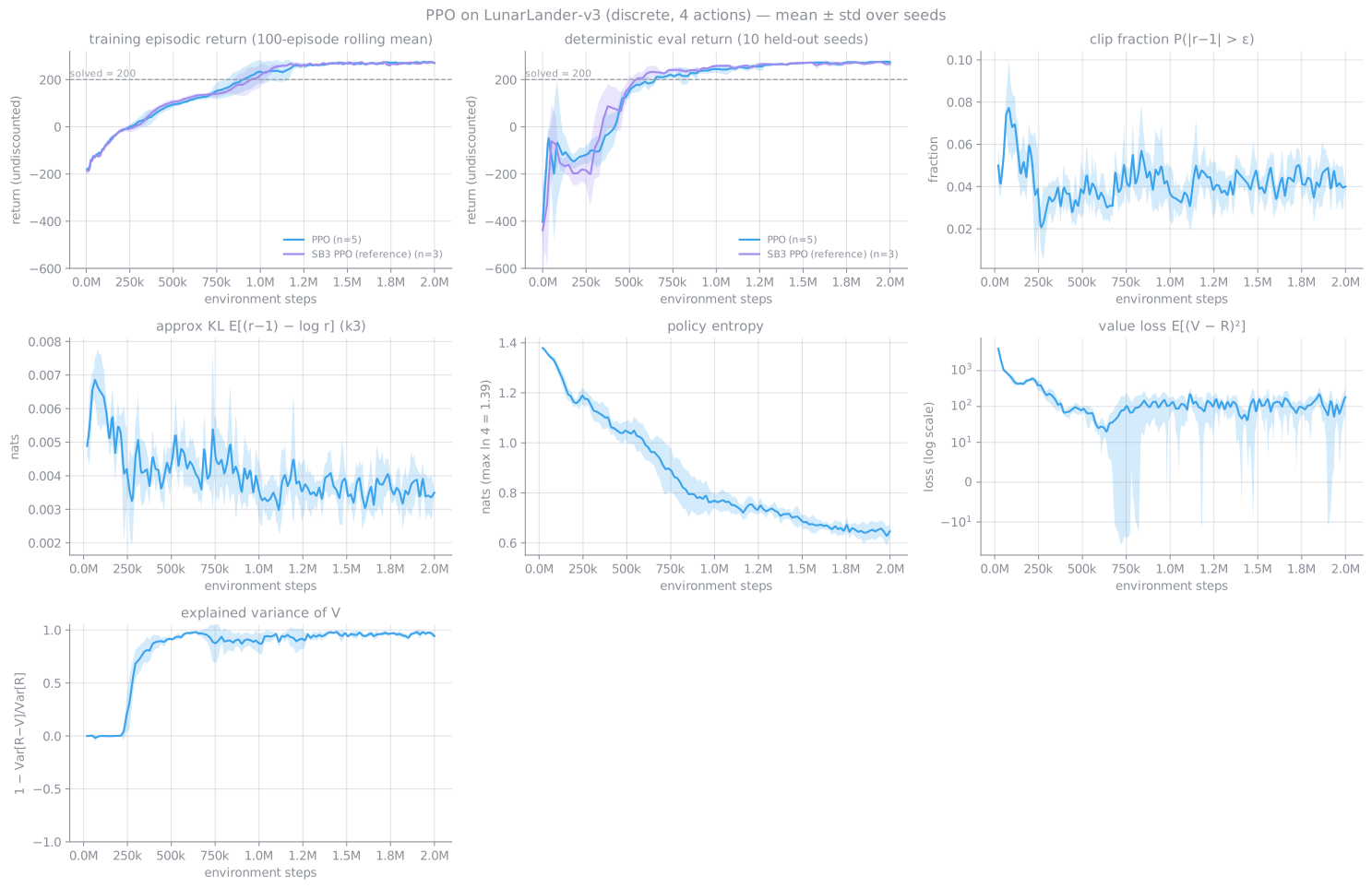
A2C takes one gradient step per batch and has nothing to stop that step from being too large. PPO (Schulman et al., 2017) fixes both problems with one device: a clipped importance ratio that makes it safe to take about a thousand minibatch steps on the same 16,384 transitions. This page derives the clip from TRPO's trust region, works through exactly what it does to the gradient, and explains each diagnostic ppo.py logs. 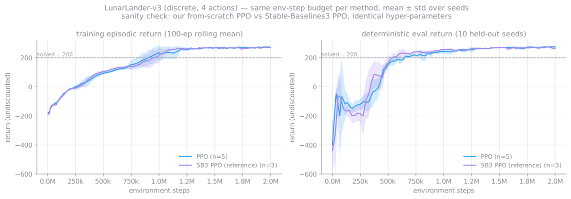On this machine PPO won outright on both action spaces and reproduced Stable-Baselines3 to within 2 points.

Shared derivations (policy-gradient theorem, baselines, GAE) are on the RL overview, cited as (overview n). The on-policy/off-policy argument for why the ratio is needed at all is on its own page. Numbers marked measured are from 5 seeds on this machine.

1 · The problem PPO solves: TRPO's trust region

Suppose we have collected data with a policy $\pi_{\theta_\text{old}}$ and want to improve it by more than one small step. The performance-difference lemma (Kakade & Langford, 2002) states exactly how much better a new policy $\pi$ is:

$$ J(\pi) - J(\pi_{\theta_\text{old}}) = \frac{1}{1-\gamma}\, \mathbb{E}_{s\sim d^{\pi},\,a\sim\pi}\big[A^{\pi_{\theta_\text{old}}}(s,a)\big] \tag{1} $$

where $d^{\pi}$ is the normalised discounted state distribution of the new policy, which we have no samples from. Replacing it with $d^{\pi_{\theta_\text{old}}}$ and rewriting the action expectation by importance sampling gives the surrogate objective:

$$ L_{\theta_\text{old}}(\theta) = \mathbb{E}_{s,a\sim\pi_{\theta_\text{old}}}\big[\,r(\theta)\,\hat A\,\big], \qquad r(\theta) = \frac{\pi_\theta(a\mid s)}{\pi_{\theta_\text{old}}(a\mid s)} \tag{2} $$

$r(\theta)$ is the importance ratio: how much more (or less) likely the new policy is to take the action that was actually taken. At $\theta = \theta_\text{old}$, $r = 1$ and $\nabla_\theta L = \mathbb{E}[\nabla_\theta\log\pi_\theta\,\hat A]$, which is the ordinary policy gradient. So (2) matches the true objective to first order. The approximation $d^\pi \approx d^{\pi_\text{old}}$ is only trustworthy while the two policies stay close, and TRPO (Schulman et al., 2015) makes that explicit as a constraint:

$$ \max_\theta\; L_{\theta_\text{old}}(\theta) \quad \text{s.t.}\quad \mathbb{E}_{s}\Big[D_\mathrm{KL}\big(\pi_{\theta_\text{old}}(\cdot\mid s)\,\big\Vert\,\pi_\theta(\cdot\mid s)\big)\Big] \le \delta \tag{3} $$

The theory behind (3) is a lower bound on $J(\pi)$ that subtracts a penalty proportional to the maximum KL (derived on the on-policy page, eq. 6). TRPO solves (3) with a second-order method: a conjugate-gradient solve against the Fisher information matrix, then a line search. That works, but it is complicated, it does not fit easily with shared networks or dropout, and each update is expensive.

2 · The clipped surrogate

PPO replaces the hard constraint with a modification of the objective itself, so that plain SGD can be used. With clip parameter $\epsilon$ ($\epsilon = 0.2$ here) and advantage estimate $\hat A_t$:

$$ L^{\text{CLIP}}(\theta) = \mathbb{E}_t\Big[\min\Big(r_t(\theta)\,\hat A_t,\; \operatorname{clip}\big(r_t(\theta),\,1-\epsilon,\,1+\epsilon\big)\,\hat A_t\Big)\Big] \tag{4} $$

The first argument of the min is the unclipped surrogate (2). The second is the same with the ratio clamped to $[0.8, 1.2]$. Taking the minimum makes $L^{\text{CLIP}}$ a pessimistic lower bound on the unclipped surrogate: when clipping would make the objective look better, the clipped version wins the min; when it would make it look worse, the unclipped version wins. That asymmetry is the whole design.

2.1 What the clip does, case by case

Write $g_t = \nabla_\theta r_t = r_t\,\nabla_\theta\log\pi_\theta(a_t\mid s_t)$. Per sample, the gradient of (4) is either $g_t\hat A_t$ (the unclipped term is active) or exactly zero (the clipped term is active, and it is constant in $\theta$). There are four regions:

Advantage	Ratio	Active term in the min	Gradient	Meaning
$\hat A \gt 0$ (good action)	$r \le 1+\epsilon$	$r\hat A$	$g\hat A$, pushes $r$ up	Make the good action more likely…
$\hat A \gt 0$	$r \gt 1+\epsilon$	$(1+\epsilon)\hat A$	0	…but stop once it is already 20 % more likely than before
$\hat A \lt 0$ (bad action)	$r \ge 1-\epsilon$	$r\hat A$	$g\hat A$, pushes $r$ down	Make the bad action less likely…
$\hat A \lt 0$	$r \lt 1-\epsilon$	$(1-\epsilon)\hat A$	0	…but stop once it is already 20 % less likely

Two cells are missing from the clipped region, and they matter. If $\hat A \gt 0$ and $r \lt 1-\epsilon$ (an earlier minibatch step accidentally made a good action less likely), the unclipped term $r\hat A$ is smaller, so it wins the min and its gradient is still active, pulling the action back up. Likewise for $\hat A \lt 0$ and $r \gt 1+\epsilon$. The clip removes the incentive to move further in the direction that already helps, but it never stops the correction of a move in the wrong direction. The figure below shows the per-sample objective as a function of $r$.

Per-sample $L^{\text{CLIP}}$ against the ratio $r$ (solid), with the unclipped $r\hat A$ (dashed) where they differ. For $\hat A \gt 0$ the objective goes flat above $1+\epsilon$. For $\hat A \lt 0$ it goes flat below $1-\epsilon$. On the other side of 1 the slope is unchanged in both cases. Schematic, after Fig. 1 of Schulman et al. (2017).

The clip is a per-sample trust region, not a global one. It does not bound the KL. A minibatch step moves the shared network weights, so it changes the ratio on every sample, including samples whose gradient has already been switched off. Ratios can and do drift past $1\pm\epsilon$. This is why PPO implementations log the KL and the clip fraction (§4): they show whether "proximal" actually held.

3 · The full loss, as implemented

ppo.py minimises, per minibatch of 64 transitions,

$$ \mathcal L(\theta,\psi) = -L^{\text{CLIP}}(\theta) + c_v\,\mathbb{E}_t\big[(V_\psi(s_t) - R_t)^2\big] - c_e\,\mathbb{E}_t\big[\mathcal H[\pi_\theta(\cdot\mid s_t)]\big], \qquad c_v = 0.5,\; c_e = 0.01 \tag{5} $$

with $\hat A_t$ and $R_t = \hat A_t + V_{\psi_\text{old}}(s_t)$ from GAE($\gamma = 0.999$, $\lambda = 0.98$) (overview 12–13). The relevant lines:

log_ratio = logp - b_logp[mb] # log pi_theta - log pi_old, [64] ratio = log_ratio.exp() # r_t(theta), eq. (2) A = b_adv[mb] A = (A - A.mean()) / (A.std() + 1e-8) # per-minibatch advantage normalisation pg_loss = -torch.min(ratio * A, ratio.clamp(1 - a.clip_eps, 1 + a.clip_eps) * A).mean() # -L^CLIP, eq. (4) v_loss = ((critic(b_obs[mb]) - b_ret[mb]) ** 2).mean() # value clipping OFF loss = pg_loss + a.vf_coef * v_loss - a.ent_coef * dist.entropy().mean() # eq. (5)

3.1 Advantage normalisation

Each minibatch's advantages are standardised to zero mean and unit variance before entering (4). The effect on the gradient's direction is small, since it amounts to subtracting a constant baseline and rescaling. The effect on its size is large. Raw GAE advantages in LunarLander range over hundreds of reward units early on and a few units late, and normalisation makes the effective step size roughly invariant to that. It also means the clip at $\epsilon = 0.2$ has the same meaning throughout training. The cost is a small bias: the mean is estimated from only 64 samples.

3.2 Value clipping: off, deliberately

The PPO2 reference code also clips the value update: $\max\big((V_\psi - R)^2,\ (V_{\psi_\text{old}} + \operatorname{clip}(V_\psi - V_{\psi_\text{old}}, -\epsilon, \epsilon) - R)^2\big)$. It is off here, for two reasons. Andrychowicz et al. (2021) found it neutral to harmful across their large study. And the clip range is in reward units: with $\epsilon = 0.2$ and returns of $O(100)$, the critic could move by at most 0.2 per update, which would effectively freeze it. The measured outcome supports the choice: explained variance reached 0.94–0.99 at the end of training on every seed.

3.3 Reusing data, counted

One rollout is $N \times T = 16 \times 1024 = 16{,}384$ transitions. It is shuffled and swept 4 times in minibatches of 64, giving 1,024 Adam steps on the same data, and then discarded. The 2M-step budget is therefore 123 rollouts (the last one runs slightly past 2M) and about 126k gradient steps. Compare A2C: 15,625 rollouts of 128, with one step each. Without the clip, 1,024 steps on fixed data would overfit the batch and drive the ratios far from 1. With the clip, each sample switches itself off once it has had its effect.

3.4 Training loop, step by step

One PPO iteration. The rollout is collected with gradients off, so $\pi_{\theta_\text{old}}$ is frozen into logp_old; GAE runs once over the whole buffer; then the same 16,384 transitions are reused for 1,024 clipped minibatch steps before being discarded.

# PPO TRAINING (ppo.py; --continuous switches the actor) equations refer to this page # N = 16, T = 1024 -> 16,384 transitions / rollout; K = 4 epochs; minibatch 64 -> 256 per epoch # gamma 0.999, lambda 0.98, eps 0.2, Adam(lr 3e-4, eps 1e-5), c_v 0.5, c_e 0.01, clip-norm 0.5 actor pi_theta : discrete 8 -> 64 -> 64 -> 4 logits (4,996 params) continuous 8 -> 64 -> 64 -> 2 means + log_sigma in R^2 = 0 (4,868 params) critic V_psi : 8 -> 64 -> 64 -> 1 (4,801 params) opt = Adam(params(actor) + params(critic)) s = envs.reset() # [16, 8] while env_steps < budget: # 2M discrete, 1M continuous # (a) ROLLOUT with gradients OFF: this freezes pi_old = pi_theta for t in 0 .. 1023: dist = pi_theta(s) # Categorical(logits [16,4]) | Normal(mu [16,2], sigma [2]) a = dist.sample() # [16] | [16, 2] buf.logp_old[t] = dist.log_prob(a) # [16] (Gaussian: summed over the 2 action dims) buf.V_old[t] = V_psi(s) # [16] s', r, term, trunc = envs.step(a) # continuous: env receives clip(a, -1, 1) r[trunc] += gamma * V_psi(final_obs[trunc]) # bootstrap the time limit buf.obs[t], buf.act[t], buf.r[t], buf.done[t] = s, a, r, term OR trunc s = s' # (b) GAE once over the whole [1024, 16] buffer (overview eq. 13) A, R = compute_gae(buf.r, buf.V_old, buf.done, V_psi(s), 0.999, 0.98) # [1024, 16] each flatten every buffer to 16,384 rows # obs [16384, 8] # (c) K = 4 epochs x 256 minibatches = 1,024 Adam steps on the SAME data for epoch in 1 .. 4: for idx in randperm(16384).split(64): dist = pi_theta(obs[idx]) logr = dist.log_prob(act[idx]) - logp_old[idx] # [64] rho = exp(logr) # eq. (2) Ahat = (A[idx] - mean(A[idx])) / (std(A[idx]) + 1e-8) # section 3.1 L_clip = mean(min(rho * Ahat, clip(rho, 0.8, 1.2) * Ahat)) # eq. (4) L_V = mean((V_psi(obs[idx]) - R[idx])^2) # value clipping OFF loss = -L_clip + 0.5 * L_V - 0.01 * mean(dist.entropy()) # eq. (5) Adam step on actor + critic, ||g|| clipped to 0.5 log approx_kl = mean((rho - 1) - logr) # k3, eq. (6) log clip_frac = mean(|rho - 1| > 0.2) log explained_var = 1 - Var[R - V_old] / Var[R] discard the buffer # it is now off-policy

Compare the listing with A2C's. The rollout runs under no_grad, so the policy that collected the data survives only as the stored logp_old. That number is what makes the ratio in (2) computable after the weights have moved. Advantages are computed once per rollout with the old critic, and the 1,024 minibatch steps then reuse them unchanged.

3.5 Inference

# PPO INFERENCE (common.evaluate) actor = load("best.pt"); actor.eval(); torch.no_grad() # critic, optimiser, buffer discarded s = env.reset(seed = q) # [8] repeat until term or trunc (at most 1,000 steps): discrete: a = argmax(logits(s)) # [4] -> int continuous: a = clip(mu_theta(s), -1, 1) # [2] Gaussian MEAN; sigma is ignored s, r, term, trunc = env.step(a) # cost: 92 us (categorical) / 99 us (Gaussian) per step on one CPU thread at batch 1, measured under load

Ignoring $\sigma$ at inference is the whole story of §7. The continuous policy trains with $\sigma \approx 1$ and is deployed with $\sigma = 0$. Those two controllers score 144–156 and 260–268 respectively.

4 · Diagnostics, and what each one means

4.1 Approximate KL: the k1, k2 and k3 estimators

The quantity we want to monitor is $D_\mathrm{KL}(\pi_\text{old}\Vert\pi_\theta) = \mathbb{E}_{a\sim\pi_\text{old}}[-\log r]$, estimated from the stored actions, which were sampled from $\pi_\text{old}$. Schulman (2020) compares three single-sample estimators, writing $r = \pi_\theta(a)/\pi_\text{old}(a)$:

Name	Estimator	Unbiased?	Always ≥ 0?	Variance
k1	$-\log r$	yes	no: individual samples are negative half the time	high
k2	$\tfrac12(\log r)^2$	no (exact only to second order)	yes	low
k3 (logged)	$(r - 1) - \log r$	yes	yes	low

k3 is k1 plus the control variate $(r-1)$, which has zero mean under the sampling distribution, because $\mathbb{E}_{a\sim\pi_\text{old}}[r] = \sum_a \pi_\text{old}(a)\,\pi_\theta(a)/\pi_\text{old}(a) = 1$. So:

$$ \mathbb{E}_{\pi_\text{old}}\big[(r-1) - \log r\big] = 0 + D_\mathrm{KL}(\pi_\text{old}\Vert\pi_\theta) \tag{6} $$

Non-negativity holds sample by sample, because $\log x \le x - 1$ for all $x \gt 0$, with equality only at $x = 1$. The same estimator in the other KL direction is GRPO's KL penalty; its derivation is on the GRPO page. ppo.py logs k3 as approx_kl, averaged over all 1,024 minibatch steps of each rollout, and also over the last epoch only:

stats["approx_kl"].append(((ratio - 1) - log_ratio).mean().item()) # k3, eq. (6) stats["clip_frac"].append(((ratio - 1).abs() > a.clip_eps).float().mean().item()) # fraction outside [0.8, 1.2]

Two caveats. The ratio inside each minibatch is computed before that minibatch's step, so the logged value slightly lags the final policy. And it is averaged over states from $\pi_\text{old}$, which is the expectation TRPO's constraint (3) uses, not the maximum its bound needs.

4.2 Clip fraction

The fraction of samples with $|r - 1| \gt \epsilon$, i.e. those currently outside the trust region. Near 0 means the clip never binds, so PPO behaves like multi-epoch A2C. Large values (above roughly 0.3) mean the policy is moving so far per rollout that most samples no longer contribute, and the learning rate or number of epochs should come down.

4.3 Explained variance

$\mathrm{EV} = 1 - \operatorname{Var}[R - V_\psi]/\operatorname{Var}[R]$, computed over each rollout (common.explained_variance). 1 means the critic predicts the return targets perfectly, 0 means it does no better than a constant, and negative means worse than a constant. Because the advantages are built from $V_\psi$, a low EV means noisy advantages, so it is the first thing to check when PPO stops improving.

5 · Hyper-parameters as run

Parameter	Value	Source
N envs × T	16 × 1024 = 16,384 / rollout	rl-baselines3-zoo LunarLander
Epochs × minibatch	4 × 64 → 1,024 Adam steps / rollout	zoo
$\gamma$, $\lambda$	0.999, 0.98	zoo; long horizon
Clip $\epsilon$	0.2	paper default
Optimiser	Adam lr 3e-4, ε 1e-5, constant	zoo / paper
$c_v$, $c_e$, grad clip	0.5, 0.01, 0.5	zoo
Value clipping	off	§3.2
Networks	separate 2×64 tanh: actor 4,996 (Gaussian 4,868), critic 4,801 params	`common.py`
Budget	2M steps discrete, 1M continuous	same as the other methods on each env

6 · Results, discrete (measured)

	seed 0	seed 1	seed 2	seed 3	seed 4	Summary
Final policy, 50 held-out eps	280.5	273.3	276.4	274.7	274.7	275.9 ± 2.5, 99.6 % solved
approx KL (k3) median / max	0.0038 / 0.0101	0.0036 / 0.0089	0.0038 / 0.0078	0.0043 / 0.0088	0.0039 / 0.0076	p99 ≤ 0.0081
Clip fraction median / max	0.041 / 0.090	0.038 / 0.121	0.041 / 0.082	0.045 / 0.093	0.040 / 0.090
Explained variance, end	0.98	0.94	0.98	0.99	0.95
Entropy, first → last	1.38 → 0.62	1.38 → 0.60	1.38 → 0.66	1.38 → 0.69	1.38 → 0.63	max ln 4 = 1.39

Steps to the first periodic eval ≥ 200: 612,762 on average (5/5 seeds). Wall-clock 946 s per seed at 2,134 env steps/s, with 13 jobs sharing the machine. Best-checkpoint eval 275.7 ± 2.6, the same as the final policy within noise. That is itself a result: unlike A2C, PPO did not degrade. The largest per-rollout KL in all 5 discrete runs was 0.0101, and no KL spikes or policy collapses occurred in any of the 10 PPO runs (discrete and continuous). With 1,024 steps per batch, the clip held the policy change per rollout to about 0.004 nats at the median.

PPO training curves on discrete LunarLander with KL, clip fraction, entropy and explained variance, plus the SB3 reference curve — **PPO on discrete LunarLander-v3**, 2M steps, 5 seeds, measured on this machine. Training return is the 100-episode rolling mean of sampled-action episodes. Evaluation is deterministic (argmax) on 10 held-out seeds every 25k steps. The diagnostic panels show the k3 approximate KL, the clip fraction, the entropy and the explained variance per rollout. The SB3 reference curve is overlaid.

6.1 Sanity check against Stable-Baselines3

A from-scratch implementation can be subtly wrong and still learn something. To rule that out, SB3's PPO was run with identical hyper-parameters, 3 seeds, as a reference only (never as the implementation): 274.0 ± 0.6 against our 275.9 ± 2.5 on the same 50 held-out seeds, first eval ≥ 200 at 525,008 steps against our 612,762, and overlapping learning curves. Our PPO is not broken. SB3's wall-clock (1,708 s) is not comparable: it ran under different load and threading.

Our PPO vs Stable-Baselines3 PPO evaluation curves — **From-scratch PPO (5 seeds) vs Stable-Baselines3 PPO (3 seeds)**, same hyper-parameters, deterministic evaluation, measured on this machine. The bands overlap throughout.

6.2 The PPO controller, flown

PPO (discrete), seed 0 best.pt, deterministic (argmax) policy, recorded on this machine. Flown on a pool of 24 held-out video seeds (3,000,000,000 onward): 24 / 24 score ≥ 200 and all 24 land. Because no pool episode failed, the video shows 4 successful episodes: 244, 271, 282 and 289, all landed. 640×400 H.264, 23.5 s. A 1920×1080 master exists for YouTube but is not deployed with the site.

6.3 Learning progression from the same starts

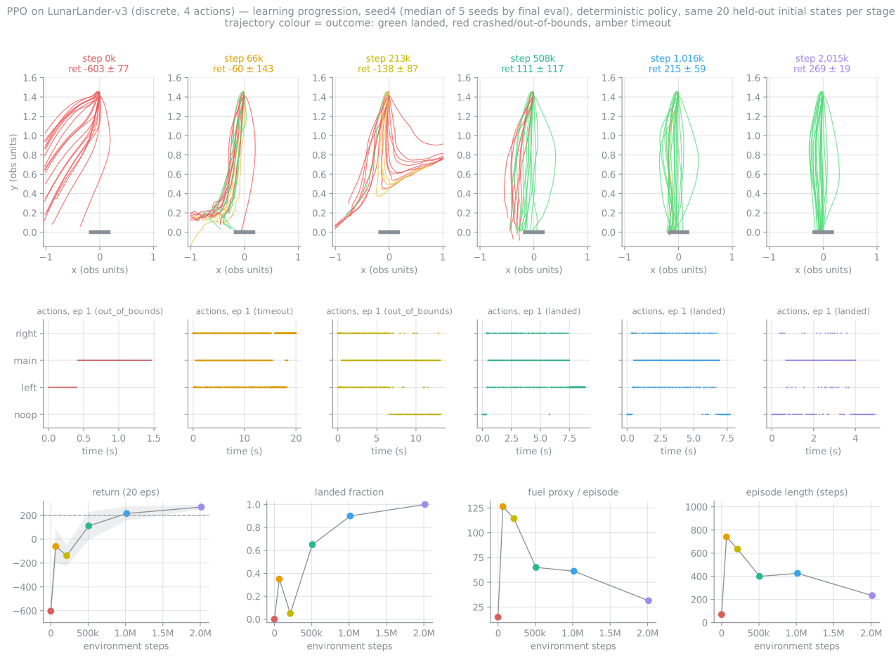
Median seed by final eval (seed 4), deterministic, the same 20 held-out starts at each stage. Mean return / fraction landed: −603 / 0 % → −60 / 35 % → −138 / 5 % → 111 / 65 % → 215 / 90 % → 270 / 100 % at 0 / 2.5 / 10 / 25 / 50 / 100 % of training. Progress is not monotone: on this seed the landed fraction fell from 35 % to 5 % between the 2.5 % and 10 % snapshots before recovering. Fuel use and episode length also fall as the policy improves. The fuel proxy goes from 126 at 65k steps to 31 at the end, and episode length from 740 to 234 steps. It learns to land quickly rather than hover.

PPO learning progression: trajectories from the same 20 held-out starts at six training stages — **PPO progression**, seed 4 (median by final eval), deterministic policy, the same 20 held-out initial states at 0, 2.5, 10, 25, 50 and 100 % of 2M steps, measured on this machine.

PPO progression video: seed 4, deterministic, one held-out start replayed with each stage's snapshot. 640×400 H.264, 21.0 s, recorded on this machine. 1080p master kept for YouTube, not deployed.

7 · Continuous actions, and a gotcha in the training curve

With --continuous the actor becomes a diagonal Gaussian $\pi_\theta(a\mid s) = \mathcal N\big(\mu_\theta(s),\ \operatorname{diag}(\sigma^2)\big)$ with a state-independent learned $\log\sigma \in \mathbb R^2$ initialised to 0, i.e. $\sigma = 1$ per action dimension. The environment receives $\operatorname{clip}(a, -1, 1)$, and the log-probability is that of the unclipped sample. Everything else in (5) is unchanged. It is PPO-continuous that serves as the like-for-like comparison for DDPG.

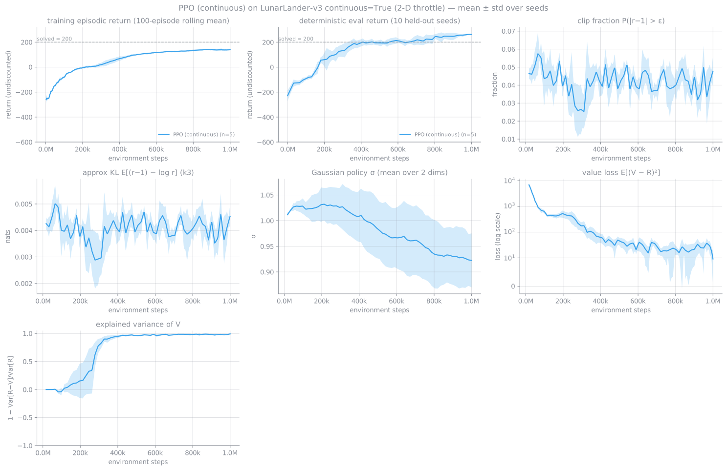
Measured: final eval 265.0 ± 2.9, 100 % of 250 episodes solved, first eval ≥ 200 at 419,430 steps (5/5), 511 s per seed. Approximate KL max 0.0052–0.0064 across seeds, clip fraction median 0.041–0.045, explained variance 0.97–0.99 at the end.

The training curve understates this controller by more than 100 points. The rolling mean of training returns stays near 150 and never crosses 200, while every deterministic evaluation from mid-training on does. The cause is that the Gaussian's $\sigma$ hardly moved: entropy went from 2.85 to 2.51–2.86, i.e. $\sigma \approx 1$ per dimension throughout. My reading is that the entropy bonus ($c_e = 0.01$) roughly balances the policy gradient's pressure to shrink $\sigma$. The mean action $\mu_\theta(s)$ became an excellent controller, while sampled actions add unit-variance noise to throttles that live in $[-1, 1]$.

Running the final policies on the same 50 held-out seeds both ways (eval_stochastic.py): the deterministic mean scores 260–268, 100 % solved, while the sampled policy scores 144–156, 0 % solved, 90–100 % timeouts. The noisy lander hovers until the time limit. For discrete PPO the two agree (273–280 deterministic vs 269–279 sampled), because its entropy did fall, to 0.27–0.44 nats at the start states. Lesson: with a state-independent $\sigma$ that the entropy bonus keeps near its initial value, never judge a continuous-action policy by its training return.

PPO-continuous training curves: training return stays near 150 while deterministic eval exceeds 250 — **PPO on continuous LunarLander-v3**, 1M steps, 5 seeds, measured on this machine. Compare the training-return panel (sampled actions, $\sigma \approx 1$) with the deterministic-evaluation panel (Gaussian mean).

8 · Honest limitations

Still on-policy. Each transition is used 4 times and then discarded. Where environment steps are expensive, an off-policy method can be preferable, though DDPG was not more sample-efficient here.
The clip is a heuristic. It does not enforce a KL bound (§2.1). On harder tasks PPO's stability depends on implementation details (normalisation, initialisation, lr schedule, gradient clipping). Engstrom et al. (2020) showed that much of PPO's advantage over TRPO comes from those details.
Entropy versus exploitation in continuous control. The fixed coefficient that kept $\sigma$ near 1 is exactly what makes the training curve misleading. A state-dependent $\sigma$, an entropy schedule, or a target-entropy method (as in SAC) would change that behaviour. Not tested here.
One task, reference hyper-parameters. The win is on LunarLander with zoo settings, not a general claim.

9 · References

Schulman, Wolski, Dhariwal, Radford, Klimov, Proximal Policy Optimization Algorithms, arXiv:1707.06347, 2017.
Schulman, Levine, Moritz, Jordan, Abbeel, Trust Region Policy Optimization, ICML 2015.
Kakade & Langford, Approximately Optimal Approximate Reinforcement Learning, ICML 2002. Eq. (1).
Schulman, Approximating KL Divergence, blog note, 2020. The k1/k2/k3 estimators.
Andrychowicz et al., What Matters in On-Policy RL? A Large-Scale Empirical Study, ICLR 2021. Value clipping, normalisation.
Engstrom, Ilyas, Santurkar, Tsipras, Janoos, Rudolph, Madry, Implementation Matters in Deep Policy Gradients, ICLR 2020.
Raffin et al., Stable-Baselines3, JMLR 2021; and rl-baselines3-zoo. The reference implementation and hyper-parameters.

Next: GRPO, which keeps this clip but drops the critic · PPO for LLMs (RLHF) · DDPG, the off-policy comparison · back to the RL overview