
A2C — advantage actor-critic
A2C is the policy-gradient theorem with a learned baseline, run as directly as possible: 16
environments take 8 steps each, the 128 transitions produce one gradient step, and the batch is
thrown away. It is the baseline every later method on this site improves on. On LunarLander it does
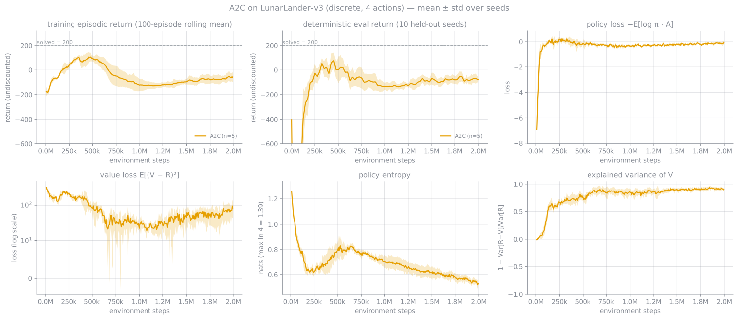
learn to land, within about half a million steps on every seed, and then it loses that skill.
This page derives the losses, explains each design choice in a2c.py, and uses the logged
diagnostics to work out why it degrades.
Prerequisites: the MDP, policy-gradient theorem, baselines and GAE are derived once on the RL overview and referred to here as (overview 7), (overview 12) and so on. Numbers marked measured come from 5 seeds run on this machine. None are paper numbers.
1 · From REINFORCE to actor-critic
REINFORCE (Williams, 1992) estimates the policy gradient (overview 7) with full Monte-Carlo returns. That is unbiased, but it must wait for each episode to finish, and its variance grows with the episode length. An actor-critic keeps two function approximators:
- the actor $\pi_\theta(a\mid s)$, the policy, here a categorical distribution $\pi_\theta(a\mid s) = \operatorname{softmax}(f_\theta(s))_a$ over the 4 discrete actions;
- the critic $V_\psi(s) \approx V^{\pi_\theta}(s)$, a learned state-value function used both as the baseline (overview 8–9) and as a bootstrap for returns that have not finished yet.
With a critic, the advantage of an action can be estimated after a handful of steps instead of after a whole episode. That is the "advantage" in A2C, and it is what makes an online, fixed-length rollout possible.
2 · The three losses
2.1 Actor: the policy-gradient surrogate
Given advantage estimates $\hat A_t$ for a batch of $B$ transitions $(s_t, a_t)$, the actor minimises
$$ \mathcal L_\pi(\theta) = -\frac{1}{B}\sum_{t} \log\pi_\theta(a_t\mid s_t)\;\operatorname{sg}\big[\hat A_t\big] \tag{1} $$where $\operatorname{sg}[\cdot]$ is stop-gradient. Differentiating (1) gives exactly minus the sample estimate of the baseline-corrected policy gradient (overview 8). The stop-gradient matters: $\hat A_t$ depends on $V_\psi$, and without it the actor's loss would also push the critic, toward whatever value makes the advantages favourable. (1) is not itself an objective whose value means anything. Only its gradient is meaningful, and only at the current $\theta$, because the samples were drawn from $\pi_\theta$. This is why the batch can be used for exactly one step (on-policy vs off-policy §2).
2.2 Critic: regression onto bootstrapped returns
The critic regresses onto a return target $R_t$ (defined in §3):
$$ \mathcal L_V(\psi) = \frac{1}{B}\sum_t \big(V_\psi(s_t) - R_t\big)^2 \tag{2} $$$R_t$ is computed with the critic's own (detached) estimates at the end of the rollout, so (2) is a semi-gradient TD method rather than true regression. The target moves as $\psi$ changes.
2.3 Entropy bonus
The entropy of the categorical policy at state $s$ is $\mathcal H[\pi_\theta(\cdot\mid s)] = -\sum_a \pi_\theta(a\mid s)\log\pi_\theta(a\mid s)$, which is between 0 (deterministic) and $\ln 4 \approx 1.386$ (uniform over the 4 actions). Subtracting it from the loss rewards the policy for staying stochastic:
$$ \mathcal L(\theta,\psi) = \mathcal L_\pi + c_v\,\mathcal L_V - c_e\,\frac{1}{B}\sum_t \mathcal H\big[\pi_\theta(\cdot\mid s_t)\big], \qquad c_v = 0.5,\; c_e = 0.001 \tag{3} $$The policy gradient alone has no reason to keep exploring. Once one action looks slightly better, (1) increases its probability, which makes it sampled more often, which reinforces it further. The entropy term is a soft counterweight to that feedback loop. Its coefficient here, 0.001, is the OpenAI baselines A2C default, and it is 10× smaller than PPO's 0.01 in this comparison. §6 shows that this matters.
3 · Advantages: n-step returns, which the code uses
a2c.py uses n-step bootstrapped returns, the original A3C/A2C estimator. In code it is
GAE with $\lambda = 1$ (--gae-lambda 1.0, overview 12–13). Within a rollout of
$n = 8$ steps, the transition at position $k \in \{0,\dots,7\}$ gets
with the sum cut at an episode boundary, where the bootstrap term is dropped. Two consequences follow from (4):
- The horizon is uneven. The first step of each window sees 7 real rewards and then the critic. The last step sees 0 real rewards, so its advantage is the pure one-step TD residual (overview 10). In terms of bias and variance, A2C is a mix of TD(0) and 8-step TD within every batch.
- "λ = 1" does not mean unbiased. With $\lambda = 1$ the GAE recursion reduces to (4), which still bootstraps from $V_\psi(s_n)$. The bias simply comes from the window edge rather than from geometric weighting.
The discount is $\gamma = 0.995$, an effective horizon of about 200 steps. The textbook 0.99 (about 100 steps) discounts the +100 landing bonus too heavily, because a landing typically arrives 200–1000 steps after the start. Keeping $\lambda = 1$ was deliberate: it keeps A2C as the classic algorithm, so the comparison with PPO (GAE $\lambda = 0.98$, clipping, minibatch epochs) isolates PPO's changes rather than retuning A2C into something else.
Time-limit truncation is bootstrapped, not treated as a crash (overview §5.1). The relevant lines:
4 · Design choices in the code
4.1 Synchronous, not A3C
A3C (Mnih et al., 2016) ran many actor-learner threads, each computing gradients on its own environment and applying them to shared parameters asynchronously, Hogwild-style. The motivation was decorrelation: different threads see different parts of the state space, which stands in for a replay buffer. A2C keeps the parallel environments but synchronises them. All 16 step in lock-step under the same $\theta$, and their transitions are stacked into a single $[8, 16]$ batch for one update.
- Correctness. In A3C a thread's gradient was computed with parameters that other threads have since changed, so updates are slightly off-policy and stale. A2C's batch is exactly on-policy.
- Efficiency. One batched forward pass of shape $[16, 8]$ uses vectorised hardware far better than 16 single-sample passes. OpenAI's baselines report found A2C matched A3C's performance at lower cost, and synchronous A2C has been the standard since.
- Determinism. With a single torch thread and synchronous vector envs, every seed's run was bit-reproducible on this machine. A second, restarted sweep gave identical final evals, for example seed 0 −83.4 and seed 1 49.7 in both (measured).
4.2 Separate actor and critic networks
Many A2C implementations share one torso with two heads. common.py builds them separately:
Measured sizes: actor 4,996 parameters, critic 4,801. The reason for separating them is the scale mismatch in (3). LunarLander returns are $O(100)$, so $\mathcal L_V$ is $O(10^3$–$10^4)$ early in training while $\mathcal L_\pi$ is $O(1)$. In a shared torso, the value gradient dominates the feature learning and $c_v$ becomes a sensitive knob. With separate networks the only coupling is the shared RMSprop step and the global gradient-norm clip at 0.5. That coupling is a real one (a large value gradient shrinks the effective actor step through the joint clip), but it is milder. Andrychowicz et al. (2021) found separate networks to be the more robust default for on-policy methods. The 0.01 gain on the policy head makes the initial logits nearly equal, so the policy starts close to uniform: the measured entropy at the first logged update is 1.23–1.36 nats, against a maximum of 1.386.
4.3 Hyper-parameters as run
| Parameter | Value | Reason |
|---|---|---|
| N envs × n steps | 16 × 8 = 128 samples / update | The classic synchronous regime: many small, single-use batches |
| Advantage | n-step returns (GAE $\lambda = 1$) | The original A3C/A2C estimator |
| $\gamma$ | 0.995 | Episodes run 200–1000 steps |
| Optimiser | RMSprop lr 7e-4, α 0.99, ε 1e-5, constant lr | A3C paper / baselines defaults |
| $c_v$, $c_e$ | 0.5, 0.001 | baselines defaults |
| Gradient-norm clip | 0.5 | baselines |
| Budget | 2,000,000 env steps = 15,625 updates | Same as PPO and GRPO |
5 · Training and inference, step by step
The diagram is one A2C update. Everything inside it happens 15,625 times in a 2M-step run, and nothing carries
over between updates except the weights. The listing below is a2c.py line by line, with tensor
shapes and the equation each line implements.
5.1 Training
Two details in the listing carry most of the method's character. The rollout keeps its autograd graph, which is legitimate only because $\theta$ does not change between collecting and updating. And the bootstrap in step (b) means that, within each window of 8, the last transition's advantage is a pure one-step TD residual while the first sees 7 real rewards.
5.2 Inference
The training policy samples; the deployed one takes the argmax. For A2C the two agree closely (sampled −118 … +62 vs argmax −120 … +50 on the 50 held-out seeds), because its entropy collapsed. §6.1 shows why that collapse is itself the problem.
6 · Results: learns, then degrades (measured)
| seed 0 | seed 1 | seed 2 | seed 3 | seed 4 | Summary | |
|---|---|---|---|---|---|---|
| Peak periodic eval (10 eps) @ step | 106 @ 600k | 152 @ 550k | 173 @ 500k | 115 @ 450k | 105 @ 325k | all peak at 325k–600k |
| Final policy, 50 held-out eps | −83.4 | 49.7 | −120.4 | −116.1 | −53.3 | −64.7 ± 62.2, 3.6 % solved |
best.pt, same 50 eps | 111.8 | 103.9 | 154.4 | 113.7 | 129.8 | 122.7 ± 18.6 |
| Entropy, first → last logged | 1.36 → 0.57 | 1.33 → 0.50 | 1.32 → 0.55 | 1.36 → 0.55 | 1.23 → 0.52 | max ln 4 = 1.39 |
| Explained variance, end | 0.90 | 0.90 | 0.96 | 0.89 | 0.90 | critic is fine |
Final eval is deterministic (argmax), on 50 held-out reset seeds never used for training or
selection. best.pt is chosen on a separate 10-seed periodic eval, so its 50-episode score is
not selection-biased. No seed's periodic eval ever reached 200. Wall-clock: 549 s per seed at
3,647 env steps/s, with 13 jobs sharing the machine.
6.1 Why it degrades: a hypothesis, tested against the logs
Three explanations are plausible. The logs support one, rule out one, and leave one only partly tested.
| Hypothesis | Prediction | What was logged | Verdict |
|---|---|---|---|
| Critic collapse: $V_\psi$ stops tracking returns, so the advantages become noise | Explained variance falls toward 0 | EV 0.89–0.96 at the end, on every seed | Ruled out |
| Entropy collapse: the policy commits to an action pattern before it is good and stops exploring the alternatives | Entropy falls well below ln 4, and the sampled and argmax policies behave the same | Training entropy 1.36 → 0.50–0.57. At the start states of the final eval the entropy is 0.08–0.24 nats, and sampled returns (−118 … +62) match argmax returns (−120 … +50) | Supported |
| Unconstrained steps: a constant lr of 7e-4 with no ratio clip lets one noisy 128-sample batch move the policy far enough to undo progress | Large per-update policy change, especially late | A per-update KL was not logged for A2C, so this is not directly measured | Consistent, untested |
The two surviving explanations reinforce each other, which is why I think both are part of the story. An unclipped policy-gradient step on a small batch has no bound on how much it moves the policy. A low-entropy policy then cannot recover from a bad move, because it rarely samples the actions that would show the move was bad. With $c_e = 0.001$ the entropy bonus contributes little against that. PPO in the same comparison has 10× the entropy coefficient and the clip, and its entropy ends at 0.60–0.69 with no collapses in 10 runs. The comparison does not separate the two effects, because PPO changes both at once. The experiments that would separate them are A2C with $c_e = 0.01$, and A2C with a linearly decaying learning rate (the baselines default). Neither was run, deliberately: the brief was reference configurations, not tuning.
6.2 The best A2C controller, flown
best.pt, deterministic (argmax) policy, recorded on this machine. This seed's
best checkpoint scores highest on the 50 final-eval seeds. It was flown on a pool of 24 video seeds
(3,000,000,000 onward, disjoint from training and evaluation). 7 / 24 pool episodes score ≥ 200
(17 landed, 4 crashed, 3 timed out). The video shows 4 episodes: three that score ≥ 200 (208, 274, 220, all
landed), then the first pool episode below 200, a −90 crash, because more than 15 % of the pool
failed. 640×400 H.264, 47.5 s. A 1920×1080 master exists for YouTube but is not deployed with the site.
6.3 Learning progression from the same starts
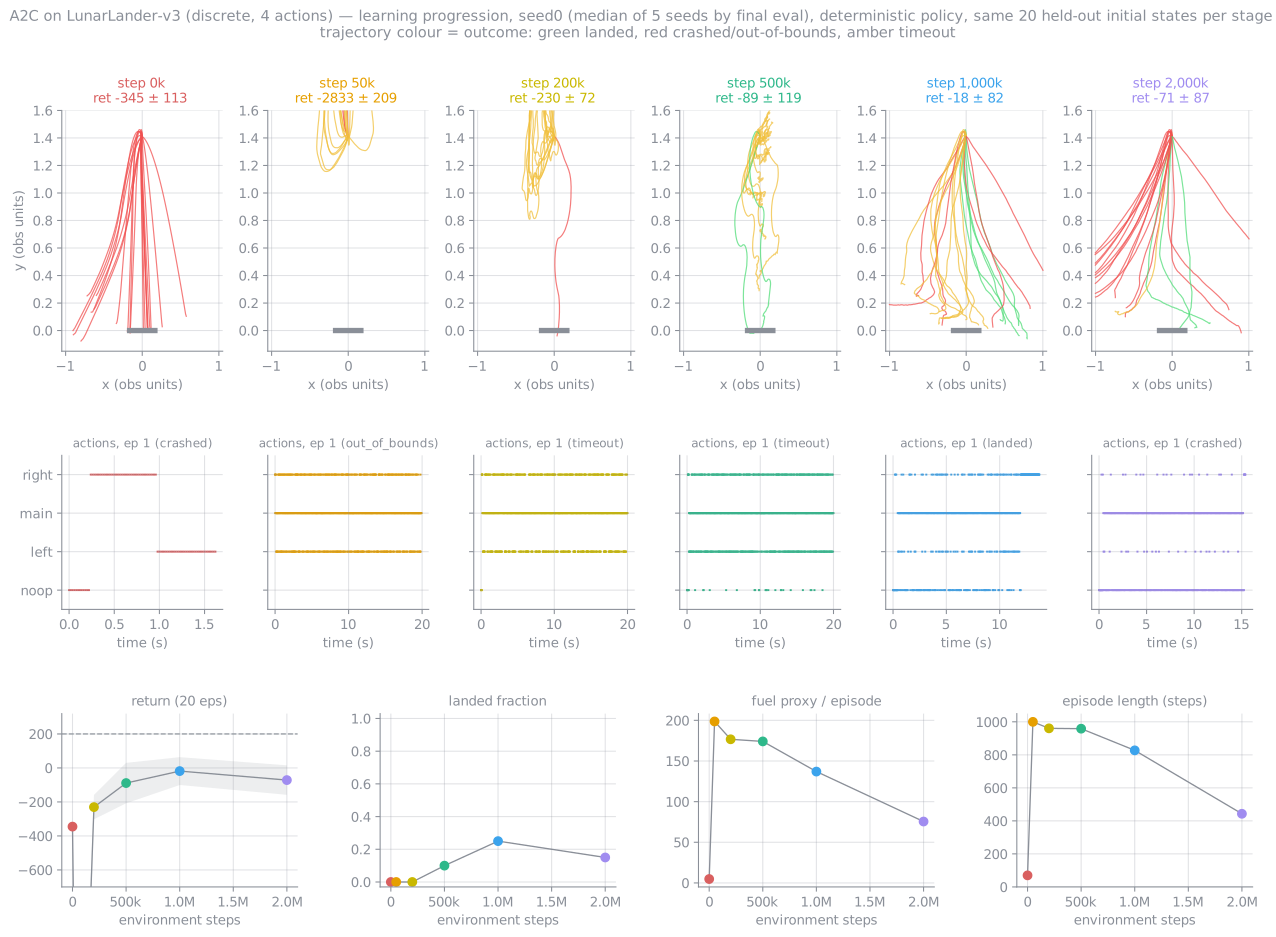
The median seed by final eval (seed 0), flown deterministically from the same 20 held-out initial states at 0 / 2.5 / 10 / 25 / 50 / 100 % of training. Mean return / fraction landed, measured: −345 / 0 % → −2,833 / 0 % → −230 / 0 % → −89 / 10 % → −18 / 25 % → −71 / 15 %. The 2.5 % stage (50k steps) is a "burn fuel and fly away" phase: 85 % of those 20 episodes run to the 1,000-step time limit, and the per-step fuel cost and the shaping penalty for drifting away accumulate into the −2,833 average. Staying airborne already beats crashing at that point; coming down has not been learned yet. The last two stages show the degradation: 25 % landed at the midpoint, 15 % at the end.
7 · Honest limitations
- Instability without a trust region. Nothing bounds the size of a policy update. §6.1 is the measured consequence. PPO's clip exists to remove it.
- Sample inefficiency. Each transition is used exactly once. That is the price of (1) being on-policy.
- Short-window bias. With $n = 8$, most of each advantage comes from the critic's bootstrap. When the critic is wrong in a systematic way, A2C has no long-horizon Monte-Carlo correction within one update.
- Untuned. These are baselines-default hyper-parameters. A larger entropy coefficient or an lr schedule might well fix the degradation. The result is a statement about the reference configuration, not about A2C's ceiling on this task.
8 · References
- Mnih, Badia, Mirza, Graves, Lillicrap, Harley, Silver, Kavukcuoglu, Asynchronous Methods for Deep Reinforcement Learning, ICML 2016. A3C and the n-step actor-critic.
- Wu, Mansimov, Liao, Grosse, Ba, Scalable trust-region method for deep RL using Kronecker-factored approximation (ACKTR), NeurIPS 2017; and the OpenAI Baselines A2C/ACKTR release, 2017. Synchronous A2C.
- Williams, Simple statistical gradient-following algorithms, 1992. REINFORCE.
- Andrychowicz et al., What Matters in On-Policy Reinforcement Learning? A Large-Scale Empirical Study, ICLR 2021. Separate networks, initialisation, entropy coefficients.
- Pardo et al., Time Limits in Reinforcement Learning, ICML 2018.
Next: PPO, A2C plus a trust region and data reuse · back to the RL overview · On-policy vs off-policy