
On-policy vs off-policy
Every RL algorithm answers one question before any other: whose actions is it allowed to learn from? On-policy methods (A2C, PPO, GRPO) may only use data generated by the policy they are currently improving, so they throw each batch away after one update. Off-policy methods (DDPG, and its descendants TD3 and SAC) learn from any transition ever collected, so they keep a replay buffer and reuse each sample hundreds of times. Neither choice is a convention. Each one falls out of a different equation, and that equation also decides how the method fails.
Companion pages: A2C · PPO ·
GRPO · DDPG. Every number marked
measured comes from the from-scratch implementations in
deeplearning/rl_lunarlander/ run on this machine (RTX 6000 Ada, 16 CPU cores), 5 seeds
per method. None are paper numbers.
1 · Two policies, not one
An agent interacts with a Markov decision process: state $s_t$, action $a_t$, reward $r_t = r(s_t, a_t)$, next state $s_{t+1} \sim P(\cdot \mid s_t, a_t)$, discount $\gamma \in [0, 1)$. The objective is the expected discounted return of a parameterised policy $\pi_\theta$:
$$ J(\theta) = \mathbb{E}_{\tau \sim \pi_\theta}\Big[\sum_{t=0}^{T} \gamma^t r_t\Big] \tag{1} $$The distinction this page is about needs two policies to be named separately:
| Symbol | Name | Role |
|---|---|---|
| $\pi$ (or $\pi_\theta$) | Target policy | The policy whose value we want and whose parameters we update. |
| $\mu$ | Behaviour policy | The policy that actually chose the actions in the data. |
2 · Why the policy gradient is on-policy
Write the trajectory probability as $p_\theta(\tau) = p(s_0)\prod_t \pi_\theta(a_t \mid s_t)\,P(s_{t+1} \mid s_t, a_t)$ and differentiate (1). The log-derivative identity $\nabla_\theta p_\theta = p_\theta \nabla_\theta \log p_\theta$ removes the unknown dynamics $P$, because they do not depend on $\theta$. With a baseline subtracted, the result is the policy-gradient theorem:
$$ \nabla_\theta J(\theta) = \mathbb{E}_{s \sim d^{\pi_\theta},\; a \sim \pi_\theta(\cdot\mid s)} \big[\nabla_\theta \log \pi_\theta(a \mid s)\; A^{\pi_\theta}(s, a)\big] \tag{2} $$Here $d^{\pi_\theta}$ is the discounted state-visitation distribution of $\pi_\theta$ and $A^{\pi}(s,a) = Q^{\pi}(s,a) - V^{\pi}(s)$ is the advantage. Read the subscript on the expectation carefully. Both the states and the actions must be drawn from the current policy. A sample $(s, a)$ collected under an older $\theta'$ is a sample from the wrong distribution, and averaging $\nabla \log \pi_\theta \cdot A$ over it estimates the gradient of a different objective.
3 · Importance sampling: reusing data, at a price
Expectations under one distribution can be rewritten under another by reweighting: $\mathbb{E}_{x\sim p}[f(x)] = \mathbb{E}_{x\sim q}\big[\tfrac{p(x)}{q(x)} f(x)\big]$. Applied to a whole trajectory, the dynamics cancel again and only action probabilities remain:
$$ \frac{p_\theta(\tau)}{p_\mu(\tau)} = \prod_{t=0}^{T} \frac{\pi_\theta(a_t\mid s_t)}{\mu(a_t\mid s_t)} = \prod_{t=0}^{T} \rho_t \tag{3} $$That is exact and unbiased, and in practice it is useless. If each per-step ratio has mean 1 and even a small spread, $\mathbb{E}[\rho_t]=1,\ \operatorname{Var}[\rho_t] = \sigma^2$, and the ratios are independent, then
$$ \operatorname{Var}\Big[\prod_{t=0}^{T}\rho_t\Big] = (1+\sigma^2)^{T+1} - 1 \tag{4} $$which grows exponentially in the horizon. A LunarLander episode is 200–1000 steps. Even with $\sigma^2 = 0.01$ and $T = 500$, the variance factor is $1.01^{501} \approx 146$. A policy that drifts a little further pushes it to millions.
3.1 PPO's answer: one-step ratios and a clip
PPO (Schulman et al., 2017) makes two approximations that turn (3) into something usable. First, it keeps only the single-step ratio and ignores the mismatch between $d^{\pi_\theta}$ and $d^{\mu}$ in the state distribution. Second, it reuses a batch for only a few epochs, so $\mu = \pi_{\theta_\text{old}}$ stays close to $\pi_\theta$. The surrogate is
$$ L^{\text{CLIP}}(\theta) = \mathbb{E}_t\Big[\min\big(\rho_t(\theta) \hat A_t,\; \operatorname{clip}(\rho_t(\theta), 1-\epsilon, 1+\epsilon)\,\hat A_t\big)\Big], \qquad \rho_t = \frac{\pi_\theta(a_t\mid s_t)}{\pi_{\theta_\text{old}}(a_t\mid s_t)} \tag{5} $$Ignoring the state-distribution shift is justified only while the policy stays close. Kakade & Langford's bound (and TRPO's version of it) makes this precise. The true improvement differs from the surrogate by a term that scales with the maximum KL between old and new policy:
$$ J(\pi_\theta) \ \ge\ J(\pi_{\theta_\text{old}}) + L_{\theta_\text{old}}(\theta) - \frac{4\gamma\,\max_{s,a}|A(s,a)|}{(1-\gamma)^2}\; \max_s D_{\mathrm{KL}}\big(\pi_{\theta_\text{old}}(\cdot\mid s)\,\|\,\pi_\theta(\cdot\mid s)\big) \tag{6} $$3.2 GRPO: on-policy without a critic
GRPO uses the same clipped ratio as (5), but replaces the learned advantage $\hat A_t$ with a group statistic. It runs $G$ rollouts from the same initial state and standardises each episode's return $R_i$ against the group: $\hat A_{i,t} = (R_i - \operatorname{mean}_j R_j)/\operatorname{std}_j R_j$ for every step $t$ of episode $i$. That estimator is valid only if the $G$ samples were drawn from the current policy, because the group mean is a Monte-Carlo estimate of $V^{\pi_\theta}(s_0)$. GRPO is therefore on-policy for a second, independent reason: its baseline is itself an on-policy estimate.
4 · Why the Bellman equation is off-policy
Now start from the action-value function instead of the return. For any policy $\pi$, $Q^\pi$ satisfies the Bellman expectation equation:
$$ Q^{\pi}(s,a) = r(s,a) + \gamma\,\mathbb{E}_{s' \sim P(\cdot\mid s,a)} \Big[\,\mathbb{E}_{a'\sim\pi(\cdot\mid s')} Q^{\pi}(s', a')\Big] \tag{7} $$Look at what the expectations range over. The outer one is over the environment's dynamics $P$, which do not depend on who chose $a$. The inner one is over the target policy at the next state, and we evaluate it ourselves. Nothing in (7) asks how $a$ was chosen. So any stored tuple $(s, a, r, s')$ is a valid sample of the outer expectation, whatever policy generated it. For a deterministic target policy $\mu_\phi$ the inner expectation collapses to a point, giving DDPG's critic target:
$$ y = r + \gamma\,(1 - d)\; Q_{w'}\big(s', \mu_{\phi'}(s')\big), \qquad \mathcal L_Q(w) = \mathbb{E}_{(s,a,r,s',d)\sim\mathcal D}\big[(Q_w(s,a) - y)^2\big] \tag{8} $$where $\mathcal D$ is the replay buffer and $w', \phi'$ are Polyak-averaged target networks. The actor is improved by the deterministic policy gradient (Silver et al., 2014):
$$ \nabla_\phi J \approx \mathbb{E}_{s\sim\mathcal D}\big[\nabla_a Q_w(s,a)\big|_{a=\mu_\phi(s)}\, \nabla_\phi \mu_\phi(s)\big] \tag{9} $$5 · How each family fails
5.1 Off-policy: over-estimation is structural
The actor in (9) climbs $Q_w$. Write the critic as truth plus zero-mean error, $Q_w = Q^\pi + \varepsilon$. The actor then lands where $Q^\pi + \varepsilon$ is largest, which is preferentially where $\varepsilon$ happens to be positive. By Jensen's inequality,
$$ \mathbb{E}_\varepsilon\Big[\max_a\big(Q^\pi(s,a) + \varepsilon(a)\big)\Big] \ \ge\ \max_a Q^\pi(s,a) \tag{10} $$and the target (8) bootstraps from exactly that over-estimated value, so the bias is copied backward through every state. Thrun & Schwartz (1993) derived this for Q-learning. Fujimoto et al. (2018) showed it persists for deterministic actor-critics, and TD3's twin critics exist to cancel it.
5.2 The deadly triad
Sutton & Barto name three ingredients that, together, can make value estimates diverge even on a simple linear problem: function approximation, bootstrapping (the target $y$ depends on $Q_{w'}$), and off-policy data. Each of the four methods here uses some subset:
| Method | Function approx. | Bootstrapping | Off-policy data | Triad complete? |
|---|---|---|---|---|
| A2C | yes | yes ($n$-step, $n=8$) | no | no |
| PPO | yes | yes (GAE, $\lambda=0.98$) | mildly (4 epochs) | no, kept in check by the clip |
| GRPO | yes | no (Monte-Carlo returns) | mildly (4 epochs) | no |
| DDPG | yes | yes (1-step TD) | yes (1M-transition replay) | yes |
Target networks (Polyak $\tau = 0.005$) and a large replay buffer are DDPG's damping against the triad. They slow the feedback loop in (8) down, but they do not break it.
5.3 On-policy: variance and wasted samples
On-policy methods avoid the triad, and the price is paid in samples and variance. A2C's single-use batches make its gradient noisy, and one bad step can undo progress with no clip to stop it. PPO's clip bounds the damage, but its data still expires after 4 epochs. GRPO pays most. It needs $G = 16$ complete episodes from each initial state before it can compute a single advantage, and the advantage then carries no temporal credit at all: every action in a crashed episode is blamed equally.
6 · Data reuse, counted
The cleanest way to compare the two families is to count how many gradient updates each environment transition contributes to. These ratios come straight from the hyper-parameters actually used:
| Method | Samples per update cycle | Gradient steps per cycle | Gradient steps per env step | Times each sample is used |
|---|---|---|---|---|
| A2C | $16 \times 8 = 128$ | 1 (full batch) | $1/128$ | 1 |
| PPO | $16 \times 1024 = 16{,}384$ | $4 \times 16384/64 = 1024$ | $1/16$ | 4 |
| GRPO | $4 \times 16$ episodes $\approx$ 6k–60k | $4 \times n/64$ | $1/16$ | 4 |
| DDPG | 1 (then sample 256 from buffer) | 1 | 1 | $\approx 256 \cdot \tfrac{T - T_0}{T} \approx$ 250 on average |
DDPG's figure: after the $T_0 = 10^4$-step warm-up it draws 256 transitions from the buffer on each of the remaining $T - T_0 = 990{,}000$ steps. That is $2.5\times10^8$ draws over at most $10^6$ stored transitions, so each one is replayed about 250 times. Older transitions are replayed more, because they have been in the buffer longer.
7 · Training and inference, step by step
The pseudo-code below is a line-by-line summary of the four training scripts that produced every
number on this page (a2c.py, ppo.py, grpo.py,
ddpg.py). Hyper-parameters are the values that actually ran, not suggestions. Tensor
shapes are written [dim, dim, …]. Comments start with # and point
back to the equation each step implements. The on-/off-policy split is visible in the structure:
the first three scripts have a collect → update → discard loop, and DDPG has a
step → store → sample old data → update loop.
7.1 Shared notation and networks
| Symbol | Value here | Meaning |
|---|---|---|
D_obs | 8 | Observation: x, y, vx, vy, angle, angular rate, left-leg contact, right-leg contact |
A | 4 | Discrete actions: no-op, left engine, main engine, right engine |
D_act | 2 | Continuous action: main throttle, lateral throttle, each in [−1, 1] |
N | 16 | Parallel environments (A2C, PPO) |
T_max | 1000 | Time-limit truncation per episode (50 Hz → 20 s) |
| Network | Layers (input → output) | Activation | Parameters | Used by |
|---|---|---|---|---|
| Categorical actor πθ | 8 → 64 → 64 → 4 logits | tanh | 4,996 | A2C, PPO, GRPO |
| Gaussian actor πθ | 8 → 64 → 64 → 2 means, + logσ [2] | tanh | 4,868 | PPO-continuous |
| Value critic Vψ | 8 → 64 → 64 → 1 | tanh | 4,801 | A2C, PPO |
| Deterministic actor μφ | 8 → 400 → 300 → 2, then tanh | ReLU | 124,502 | DDPG |
| Q critic Qw | concat(8, 2) = 10 → 400 → 300 → 1 | ReLU | 125,001 | DDPG |
The on-policy networks use orthogonal initialisation (gain √2 on hidden layers, 0.01 on the policy head so the initial policy is near-uniform, 1.0 on the value head). DDPG uses PyTorch's default initialisation, as in the TD3 reference code. GRPO trains only the 4,996-parameter actor, with no critic at all.
7.2 A2C: one gradient step per 128 transitions
7.3 PPO: 16,384 transitions, reused 4 times inside the clip
7.4 GRPO: 64 whole episodes, no critic, group-relative advantage
7.5 DDPG: one gradient step per env step, on 256 old transitions
7.6 Inference: running the trained controller
At deployment the four methods collapse into one loop. Only the actor is kept: the value critic, the Q critic, the target networks, the reference policy and the replay buffer are training-time scaffolding and are discarded. Exploration is switched off. Every evaluation number, video and progression figure on this site uses exactly this loop.
bench_inference.py,
batch 1, torch.no_grad(), taken while 13 training jobs were loading the machine, so these
are upper bounds): 92 µs for the 4,996-parameter categorical actor, 99 µs
for the Gaussian actor, 138 µs for the 124,502-parameter DDPG actor. That is
0.5–0.7 % of the 20,000 µs control period at 50 Hz, and comparable to one
Box2D env.step() (84–88 µs). The same forward pass on the RTX 6000 Ada
takes about 590 µs. At batch size 1, kernel-launch and host↔device copy overhead
dominate, so the GPU is about 5× slower. Deploy these controllers on CPU.
8 · Measured on LunarLander
The like-for-like comparison is on the continuous action space, because DDPG cannot act in the discrete one. PPO with a Gaussian policy runs on exactly the same environment, with the same 1M-step budget, the same evaluation seeds and the same deterministic evaluation policy.
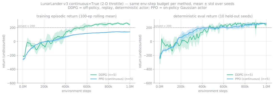
LunarLander-v3, continuous=True.
Left: 100-episode rolling training return. Right: deterministic evaluation on 10 held-out seeds.
Bands are ±1 std over 5 seeds.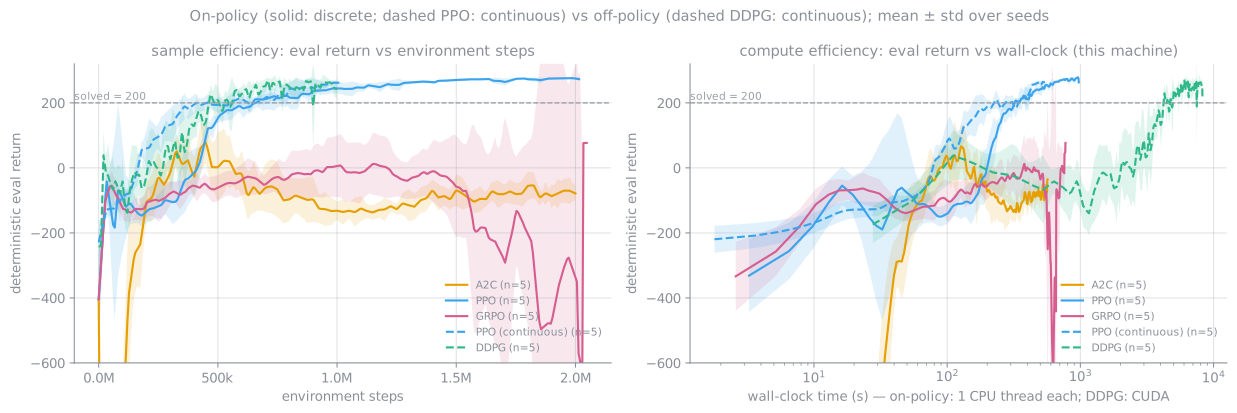
| Config | Family | Env steps | Final eval (50 eps) | Solved rate | Steps to eval ≥ 200 | Wall-clock | Env steps / s |
|---|---|---|---|---|---|---|---|
| PPO | on | 2.0M | 275.9 ± 2.5 | 99.6 % | 613k (5/5) | 946 s | 2,134 |
| A2C | on | 2.0M | −64.7 ± 62.2 | 3.6 % | never (0/5) | 549 s | 3,647 |
| GRPO | on | 2.0M | −388.9 ± 746.6 | 2.0 % | never (0/5) | 743 s | 2,735 |
| PPO (continuous) | on | 1.0M | 265.0 ± 2.9 | 100 % | 419k (5/5) | 511 s | 1,993 |
| DDPG (continuous) | off | 1.0M | 249.1 ± 27.8 | 85.6 % | 406k (5/5) | 8,249 s | 121 |
8.1 Watching both families learn
The two videos replay the same held-out initial state with the policy saved at several points in training (0 %, then roughly 2.5 %, 10 %, 25 %, 50 % and 100 %; DDPG snapshots every 50k steps, so its first non-zero stage is 10 %), for the median seed of each method. Measured over 20 held-out starts per stage, the two curves have nearly the same shape. Median-seed DDPG lands 0 % / 10 % / 80 % / 100 % at 10 / 25 / 50 / 100 % of training. PPO lands 0 % / 45 % / 100 % / 100 % at 10 / 25 / 50 / 100 %. Neither shows the "competent within a few percent of the budget" behaviour that off-policy methods are often credited with.
9 · Advantages, disadvantages, and when to use which
| On-policy (A2C, PPO, GRPO) | Off-policy (DDPG, TD3, SAC) | |
|---|---|---|
| Gradient is | An unbiased (A2C) or trust-region-approximate (PPO) estimate of $\nabla J$ itself, eq. (2)/(5) | The gradient of a learned critic, eq. (9), which is only as good as $Q_w$ |
| Sample efficiency | Low: each sample is used 1–4 times | High: each sample is replayed $\sim$250 times |
| Compute per env step | Low: 1/128 to 1/16 gradient steps | High: $\ge 1$ gradient step, bigger nets |
| Parallelism | Excellent: collection is embarrassingly parallel over envs | Awkward: the update loop is sequential |
| Stability | Good (PPO); triad avoided | Fragile; triad complete, over-estimation (10) is structural |
| Action spaces | Discrete and continuous, same code | DDPG/TD3: continuous only (needs $\nabla_a Q$) |
| Exploration | Built into the stochastic policy (entropy) | Must be bolted on (Gaussian/OU noise); a deterministic actor never explores by itself |
| Can learn from logged / human / old data | No | Yes. This is the basis of offline RL. |
| Hyper-parameter sensitivity | Moderate | High ($\tau$, noise scale, lr, buffer size, warm-up) |
10 · References
- Sutton, McAllester, Singh, Mansour, Policy Gradient Methods for RL with Function Approximation, NeurIPS 2000. The policy-gradient theorem, eq. (2).
- Kakade & Langford, Approximately Optimal Approximate RL, ICML 2002; Schulman et al., Trust Region Policy Optimization, ICML 2015. Eq. (6).
- Schulman, Wolski, Dhariwal, Radford, Klimov, Proximal Policy Optimization Algorithms, 2017. Eq. (5).
- Mnih et al., Asynchronous Methods for Deep RL, ICML 2016. A3C/A2C.
- Silver et al., Deterministic Policy Gradient Algorithms, ICML 2014. Eq. (9).
- Lillicrap et al., Continuous Control with Deep RL (DDPG), ICLR 2016.
- Fujimoto, van Hoof, Meger, Addressing Function Approximation Error in Actor-Critic Methods (TD3), ICML 2018. Over-estimation in actor-critics, and the "OurDDPG" settings used here.
- Thrun & Schwartz, Issues in Using Function Approximation for RL, 1993. Eq. (10).
- Sutton & Barto, Reinforcement Learning: An Introduction, 2nd ed., §11.3. The deadly triad.
- Precup, Sutton, Singh, Eligibility Traces for Off-Policy Policy Evaluation, ICML 2000. Per-decision importance sampling, eq. (3)–(4).
- Shao et al., DeepSeekMath, 2024. GRPO, §3.2.
Related: RL overview · A2C · PPO · GRPO · DDPG · PPO & GRPO for LLMs