
OpenEMMA — a VLM as an end-to-end driving policy
OpenEMMA is an open reproduction of Waymo's EMMA: instead of a perception stack feeding a planner, a single pretrained vision-language model is asked — in English — to look at a camera image and emit the car's future trajectory. There are no driving weights to download, because there is no training. The entire "model" is four prompts in a chain. This page derives the maths, runs it on real nuScenes data on one GPU, and reports what actually came out — including a failure mode that the standard metric completely hides.
Symbols used on this page are defined in the Nomenclature → frames, position & motion.
Sources: OpenEMMA, arXiv:2412.15208 ·
EMMA (Waymo), arXiv:2410.23262 ·
taco-group/openemma ·
nuScenes.
Every number and image below came from a run on this machine
(RTX 6000 Ada, nuScenes v1.0-mini, Qwen2.5-VL-3B-Instruct); the scripts are in
openemma/run_nuscenes_inference.py.
1 · What problem this is solving
1.1 The modular stack and its seams
A conventional autonomy stack is a pipeline: detect objects, track them, predict their futures, then plan a path. Each stage has its own training data, its own metric and its own failure modes, and every interface between them is a lossy bottleneck. A detector that outputs boxes has already thrown away the fact that the thing in the box is a construction excavator parked in the intersection rather than a car waiting at a light. The planner never sees the difference.
The end-to-end bet is that a single network mapping pixels to trajectory avoids those seams. The problem is data: driving demonstrations are expensive, and a network trained only on them has no knowledge of the world beyond what the fleet happened to encounter.
1.2 The VLM bet
EMMA's observation is that a large vision-language model has already absorbed an enormous amount of world knowledge from internet-scale pretraining. It knows what an excavator is, that a crosswalk implies pedestrians have right of way, and that orange cones mean construction. So rather than train a driving network from scratch, reformulate driving as a question answering task and let the VLM's existing knowledge do the perception.
OpenEMMA is the open reproduction of that idea using off-the-shelf open VLMs. Which leads to the single most important structural fact about it:
2 · The architecture
2.1 Four calls, one of them stateful
Each predicted frame costs four sequential VLM calls. The output of each is pasted into the prompt of the next, which is what makes this "chain-of-thought" rather than a single query:
Calls ① and ② are pure perception. Call ③ is the only part of the system with memory: the previous frame's intent is fed back in, so the model is asked to update an intent rather than invent one from scratch. Call ④ is where the language model is asked to stop talking and produce numbers.
2.2 Why the split matters
Splitting perception from control is not cosmetic. A single "look at this and give me a trajectory" prompt performs badly because the model has no budget to reason — autoregressive models do their thinking in their output tokens, so a prompt that demands numbers immediately gets numbers with no reasoning behind them. By forcing three paragraphs of description first, the numeric call has a rich textual context to condition on.
This is also the expensive part. Four calls at ~4.4 s each is 17.5 s per predicted frame, measured below. The pipeline is a research instrument, not something that runs at 10 Hz on a vehicle.
3 · The motion representation
3.1 Why not just predict (x, y)?
The obvious output format is ten future positions. OpenEMMA instead asks for ten (speed, curvature) pairs. The reason is that a language model emitting coordinates must implicitly respect a kinematic constraint it has no way to enforce: consecutive positions have to be consistent with a plausible speed and a plausible steering angle. Nothing stops a token predictor from emitting a path that teleports sideways.
Speed and curvature are the vehicle's actual control inputs — throttle and steering. Any sequence of them, however wrong, integrates to a kinematically valid path. The representation makes physical nonsense unrepresentable.
3.2 Curvature from a discrete path
To build the ground truth and the history shown in the prompt, curvature has to be estimated from three consecutive ego positions. Using the circumscribed circle of the triangle they form,
$$ \kappa = \frac{1}{R} = \frac{4A}{L_1 L_2 L_3}, $$where $A$ is the triangle's area and $L_1, L_2, L_3$ its side lengths. The sign comes from the cross product of the two leg vectors, so $\kappa > 0$ is a left turn:
$$ A = \tfrac12\left|(\mathbf p_2 - \mathbf p_1) \times (\mathbf p_3 - \mathbf p_1)\right|, \qquad \operatorname{sign}(\kappa) = \operatorname{sign}\!\big((\mathbf p_2 - \mathbf p_1) \times (\mathbf p_3 - \mathbf p_1)\big). $$Degenerate cases matter here. Three collinear points give $A = 0$ and $\kappa = 0$, which is correct. But a stationary vehicle gives $L_i \to 0$ and the expression becomes $0/0$ — so the implementation must clamp the denominator. A car waiting at a light is exactly the case that produces a divide-by-zero.
3.3 The ×100 scaling trick
Real road curvature is tiny — a comfortable lane change is around $0.01\ \text{m}^{-1}$. Asking a
language model to emit 0.0043 invites it to tokenise the leading zeros and lose precision,
and the difference between 0.004 and 0.005 is a single token with almost no
probability mass separating them. OpenEMMA therefore multiplies curvature by 100 before showing it
and divides by 100 after parsing, so the model works with numbers like 0.4 and
2.9.
It is a prompt-engineering detail with real consequences: it sets the quantisation floor of the
whole system. The model reliably emits one decimal place, so the finest curvature it can express is
$0.1 / 100 = 10^{-3}\ \text{m}^{-1}$. At 5 m/s over 5 s that is about 6 cm of lateral deviation — fine.
But it also means a prediction of -0.1 is the smallest non-zero turn the model can
name, and as we will see, that value dominates its output.
4 · From controls back to a trajectory
4.1 Unicycle integration
Given predicted speeds $v_k$ and curvatures $\kappa_k$ at $\Delta t = 0.5$ s (nuScenes keyframes are 2 Hz), the path follows the unicycle model. Curvature is yaw rate per unit distance, so yaw rate is $\dot\theta = \kappa v$:
$$ \theta_{k+1} = \theta_k + \kappa_k v_k \Delta t, \qquad \begin{bmatrix} x_{k+1} \\ y_{k+1} \end{bmatrix} = \begin{bmatrix} x_k \\ y_k \end{bmatrix} + v_k \Delta t \begin{bmatrix} \cos\bar\theta_k \\ \sin\bar\theta_k \end{bmatrix}, \qquad \bar\theta_k = \tfrac12(\theta_k + \theta_{k+1}). $$| Symbol | Meaning | Units |
|---|---|---|
| $v_k$ | Predicted speed over step $k$ | m/s |
| $\kappa_k$ | Predicted path curvature (signed, + is left) | 1/m |
| $\theta_k$ | Heading, integrated — not predicted directly | rad |
| $\bar\theta_k$ | Midpoint heading used for the position update | rad |
| $\Delta t$ | Keyframe interval | 0.5 s |
Using the midpoint heading $\bar\theta_k$ rather than $\theta_k$ is a trapezoidal rather than Euler step. On a constant-curvature arc it removes the first-order bias that otherwise makes every turn cut the corner — the same correction that appears in strapdown inertial mechanisation, for the same reason: the frame rotates during the interval over which you are integrating.
4.2 Heading error compounds — and that is the whole story
Note what the integration does to errors. A speed error enters the position once, as a displacement along the path. A curvature error enters the heading, which then rotates every subsequent displacement. Formally, a constant curvature error $\delta\kappa$ produces a heading error growing linearly in arc length $s$, and a cross-track error growing quadratically:
$$ \delta\theta(s) = \delta\kappa \cdot s, \qquad \delta y(s) \approx \tfrac12\,\delta\kappa\, s^2. $$At 5 m/s over the 5 s horizon, $s = 25$ m. A curvature error of just $0.005\ \text{m}^{-1}$ — half of one unit in the scaled representation the model emits — gives $\delta y \approx \tfrac12(0.005)(25)^2 \approx 1.6$ m, nearly a full lane width. This single sensitivity explains every bad number in §7, and it is why getting the sign of the turn right matters far more than getting the speed right.
4.3 The round-trip check
Before trusting any model output I ran a correctness gate on the representation itself: take the ground-truth future path, convert it to (speed, curvature) with §3.2, integrate it back with §4.1, and measure how far the reconstruction lands from where it started.
This is a floor. It is the error a perfect model would still incur, because it is the information destroyed by the encoding. Any reported accuracy better than this floor is a measurement artefact, not a result.
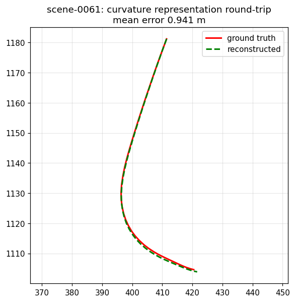
scene-0061: the reconstruction tracks the truth to 0.94 m over 5 s. The encoding is faithful here, so error measured on this scene really is the model's fault. §7.3 shows a scene where this is emphatically not the case.
5 · Drawing the prediction back into the image
The overlays below need world-frame waypoints projected into the camera. That is a chain of four transforms, each of which is a place to get a convention wrong:
$$ \mathbf p_{\text{img}} \sim K \cdot \big(T^{\text{cam}}_{\text{ego}}\big)^{-1} \cdot \big(T^{\text{ego}}_{\text{world}}\big)^{-1} \cdot \mathbf p_{\text{world}}. $$| Stage | From nuScenes | Note |
|---|---|---|
| world → ego | ego_pose (translation + quaternion) |
Per-keyframe; this is the localisation output |
| ego → camera | calibrated_sensor |
Fixed extrinsics; CAM_FRONT sits forward and ~1.5 m up |
| camera → pixels | camera_intrinsic ($K$) |
Pinhole; nuScenes CAM_FRONT is already undistorted |
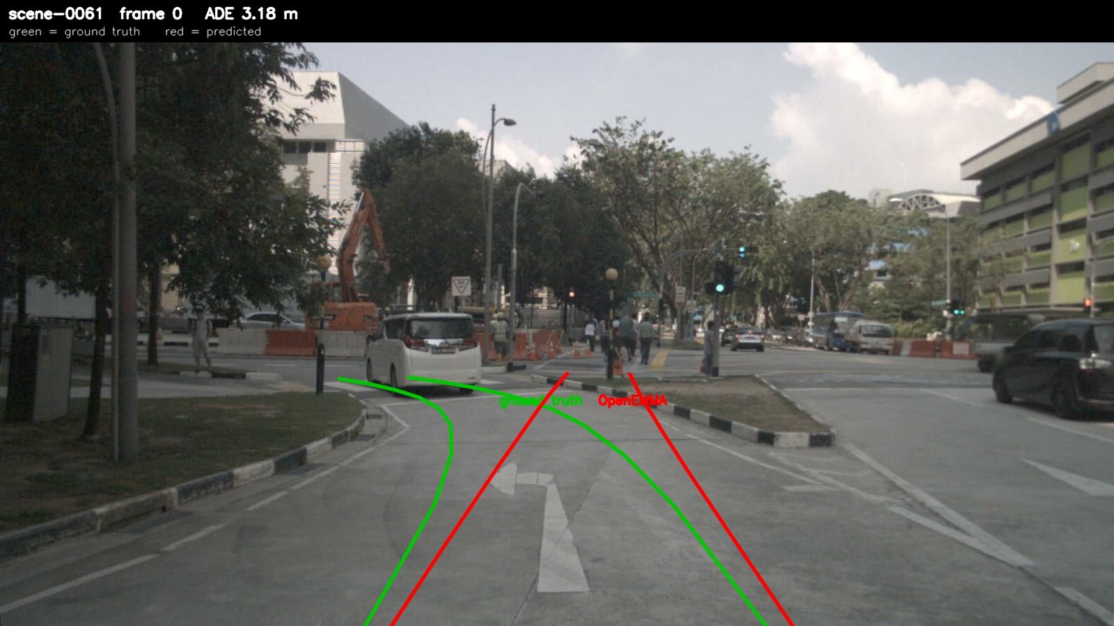
Real inference output, scene-0061 frame 0. The path is drawn as two offset rails rather than a single line, which makes the ground plane and the direction of curvature legible — a single polyline is ambiguous about which way it bends once it is foreshortened.
6 · Running it
6.1 Three defects in the upstream script
I wrote a standalone runner rather than calling the repository's main.py, because reading it
turned up three things that make it unusable as-is:
| Defect | Consequence |
|---|---|
Model path hardcoded to /root/OpenEMMA/models/… |
Only resolves on the authors' machine |
vlm_inference() defined twice (lines ~53 and ~524) |
Python keeps the second; the first — with the LLaVA and Llama branches — is dead code that silently never runs |
Scene allowlist hardcoded: if not name in ["scene-0103","scene-1077"]: continue |
--dataroot appears to work but silently evaluates two scenes |
6.2 Two dependency traps
The published requirements do not resolve to a working environment. Both failures are silent, which is what makes them worth recording:
transformers>=4.46.2with no upper bound. Pip resolves this to 5.x, which requirestorch>=2.5. On torch 2.3 it prints one line —Disabling PyTorch because PyTorch >= 2.5 is required— and then imports successfully with every model class missing. The symptom isImportError: cannot import name Qwen2_5_VLForConditionalGeneration, which looks like a model problem and is actually a torch version problem. Pinned to4.49.0.nuscenes-devkitpinsmatplotlib<3.6.0, which collides with everything else and yieldsResolutionImpossible. Installed with--no-depsand its real runtime dependencies listed explicitly.flash-attnis listed but not needed — a ~30-minute CUDA compile for no benefit at this scale.
Also worth knowing: nuScenes metadata nests one level deeper than it looks. For
v1.0-mini the correct --dataroot is the directory containing the
v1.0-mini/*.json files, which is itself named v1.0-mini. Getting it wrong gives
FileNotFoundError: …/category.json.
6.3 What it costs
| Quantity | Measured |
|---|---|
| GPU | RTX 6000 Ada (47.5 GiB) |
| Base model | Qwen2.5-VL-3B-Instruct (7.5 GB of weights) |
| Peak VRAM | 10.64 GiB — fits a 12 GB consumer card |
| Model load | 3.6 s |
| VLM calls | 96 (4 per frame × 24 frames) |
| Mean latency per call | 4.37 s |
| Per predicted frame | 17.5 s |
| Total wall clock | 440 s for 3 scenes × 8 frames |
7 · Results on real nuScenes data
7.1 The metric
Average displacement error is the mean Euclidean distance between predicted and true positions over the horizon, plus the standard snapshots at 1 s, 2 s and 3 s:
$$ \mathrm{ADE} = \frac{1}{N}\sum_{k=1}^{N} \left\| \hat{\mathbf p}_k - \mathbf p_k \right\|_2 . $$7.2 The numbers
| Scene | Content | ADE | 1 s | 2 s | 3 s | Encoding floor |
|---|---|---|---|---|---|---|
| scene-0061 | Construction, intersection, turn left | 5.66 m | 2.50 | 2.17 | 2.69 | 0.94 m |
| scene-0103 | Pedestrians, cyclist, waiting to turn | 10.94 m | 2.13 | 3.37 | 5.66 | 1.04 m |
| scene-1077 | Night, big street, exiting a sharp turn | 9.65 m | 6.51 | 7.22 | 7.95 | 9.93 m |
| Overall | 24 frames | 8.75 m | 3.71 | 4.25 | 5.43 | — |
For scale, a lane is about 3.5 m wide. An 8.75 m mean error at a 5 s horizon is several lanes — the predictions are not close.
7.3 The floor exceeds the error
My first guess was that this was a high-speed effect, since nuScenes labels scene-1077 "high speed". The data says otherwise — observed speeds over the evaluated frames run 3.1–6.3 m/s, squarely in the same range as the other two scenes. That explanation was simply wrong.
What is actually distinctive is the curvature transient. The observed history starts at $\kappa \times 100 = 7.4$ and decays to zero within ten frames: the vehicle is unwinding out of a sharp turn onto a straight road while accelerating.
The integration in §4.1 holds $\kappa_k$ constant across each 0.5 s step. That is a good approximation when curvature is steady and a poor one when it changes by several units per step — a sequence of piecewise-constant arcs cannot follow an unwinding spiral. So the representation that makes invalid paths unrepresentable (§3.1) pays for it by representing rapid curvature change badly.
The fix is in the harness, not the model: interpolate curvature linearly between samples (a clothoid segment) instead of holding it constant, or sample faster than 2 Hz. Worth stating plainly — this particular error was never the model's to begin with.
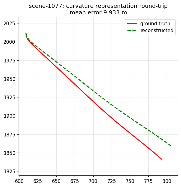
The same check as §4.3, same code, different scene. This is why the round-trip gate had to exist: without it I would have reported 9.65 m as a model result.
8 · Diagnosis — what the model actually does wrong
8.1 It turns the wrong way
ADE is a scalar that blends speed error and heading error, so it cannot tell you which is broken. I therefore checked the sign of the predicted curvature against the sign of the curvature the car was already executing — a quantity handed to the model in the prompt as observed history, so it need not infer it from pixels at all.
| Diagnostic over 24 frames | Result |
|---|---|
| Turn-direction sign flips | 11 / 19 (58%) |
| Median $|\kappa_{\text{pred}}| / |\kappa_{\text{obs}}|$ | 0.50 |
| Outputs that are perfect linear ramps in speed | 11 / 24 |
| Outputs that are perfect linear ramps in curvature | 4 / 24 |
58% sign agreement is indistinguishable from a coin flip. And the median magnitude ratio of 0.50 says that even when the direction is right, the model commits to half the turn the vehicle was already making. Combined with the quadratic error growth of §4.2, that is sufficient on its own to explain the metres of error.
8.2 The clearest single example
scene-0061 frame 5. The scene is labelled "turn left" by nuScenes, and the observed curvature history in the prompt ramps unambiguously positive — the car is already turning left, harder each step:
The model's own English intent for this frame was "maintain its current speed and continue straight ahead" — while the car was mid-left-turn through a construction zone. The perception calls described the excavator and the pedestrians correctly. The reasoning simply did not reach the numbers.
8.3 The output is a pattern, not a prediction
Look at the structure of that prediction: speed 3.5, 3.6, 3.7 … 4.4 and curvature
-0.1, -0.2, -0.3 … -1.0. Both are exact arithmetic sequences. Real vehicle motion is
never exactly linear, and 11 of 24 frames produced perfect linear speed ramps.
The -0.1 value is also telling. Per §3.3 that is the smallest non-zero curvature the
representation can express, and it is the model's default — it hedges toward the minimum
representable turn rather than committing. Seven of eight frames on scene-1077 were predicted
essentially straight.
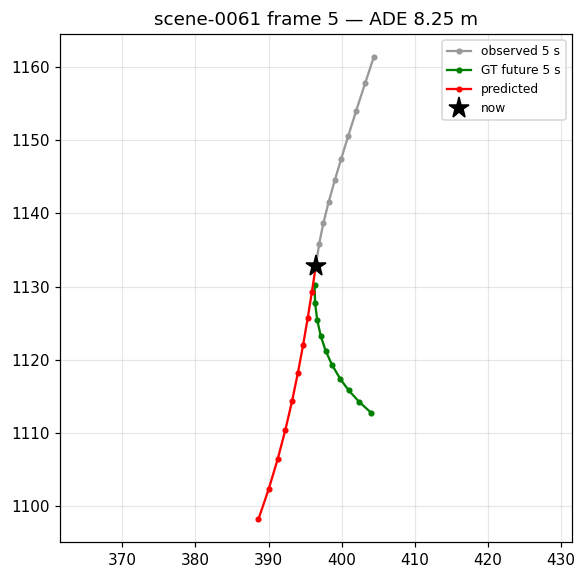
Bird's-eye view of that frame. Ground truth curves one way, the prediction ramps smoothly the other.
8.4 Why 1 s error looks respectable
The 1 s column hovers around 2–2.5 m on the two usable scenes, which is much better than the 5 s mean. This is not evidence of partial competence — it is §4.2 arithmetic. At 1 s the heading error has had almost no arc length to act over, so position is dominated by the speed estimate, which the model gets roughly right by copying the observed history. The heading error only becomes visible once $s$ grows enough for the $\tfrac12\delta\kappa s^2$ term to matter.
Which is a general warning about short-horizon metrics on integrated predictions: they measure the integration constant, not the dynamics.
9 · Training
9.1 There is nothing to fine-tune, officially
Per §1.2, upstream ships no training code. The prompt is the model. So "set up code for training" means deciding what the right training objective would be, given the failure identified above.
9.2 What the diagnosis implies about the fix
The measurements in §8 point somewhere specific. The model's perception is good — it reliably identifies the excavator, the crosswalk, the barriers. What fails is the mapping from that correct understanding to calibrated numbers. That is not a perception problem and no amount of better visual grounding will fix it.
9.3 The scaffold
train_lora.py implements supervised fine-tuning on nuScenes ego-motion with the pieces that
matter for correctness:
- Geometry and prompts imported from the inference script, so training and evaluation cannot silently disagree about curvature sign or the ×100 scale — the single most likely way to produce a model that scores well and drives wrongly.
- Label masking so the loss is computed only over assistant tokens. Without this the model spends capacity learning to reproduce the prompt.
- Frozen vision tower. Per §9.2 the deficit is not visual.
--overfit-one-batchcorrectness gate. If loss on a single batch cannot be driven to near zero, the data pipeline or the masking is wrong, and no full run will fix it. This should always be the first thing executed.
An honest caveat: nuScenes mini is 10 scenes. It is enough to validate that the plumbing works and to demonstrate overfitting on purpose; it is nowhere near enough to fix calibration. The full nuScenes trainval split, or a larger ego-motion corpus, is the real requirement.
10 · What to take away
| Claim | Verdict from this run |
|---|---|
| A pretrained VLM can describe a driving scene usefully | Supported. The CoT names the excavator, the crosswalk pedestrians, the construction barriers, unprompted and correctly |
| …and can therefore be used as a zero-shot planner | Not supported. 58% turn-direction accuracy, half-magnitude curvature, arithmetic-sequence outputs |
| Speed/curvature is a good action space for an LM | Mixed. It guarantees valid paths, but it is ill-conditioned at high speed — enough to make the metric meaningless on scene-1077 |
| Runs on accessible hardware | Supported. 10.6 GiB peak, but 17.5 s per frame |
11 · Further reading
- OpenEMMA: Open-Source Multimodal Model for End-to-End Autonomous Driving — the paper reproduced here.
- EMMA: End-to-End Multimodal Model for Autonomous Driving (Waymo) — the closed original.
- Qwen2-VL — the base model family, and the source of whatever reasoning ability the pipeline has.
- nuScenes — dataset, sensor suite and the ego-pose conventions used in §5.
- LoRA — the adaptation method in §9.3.
- ST-P3 and UniAD — trained end-to-end planners, for the comparison this page implies.
Related pages on this site: VLA & robotics for the same pixels-to-actions question in manipulation; Hyperparameter tuning for the training practices behind §9; and Optimizers for why the scaffold defaults to AdamW.