
Reinforcement learning
Four algorithms, one lander. This section derives the machinery every policy-optimisation method
shares (the MDP, the Bellman equations, the policy-gradient theorem, baselines and GAE) and then
takes A2C, PPO, GRPO and DDPG apart one at a time. Each was written from
scratch in a few hundred lines of PyTorch and trained on Gymnasium's LunarLander-v3, 5 seeds per
method, on this machine. The last page carries the same ideas over to language models, where PPO and
GRPO do most of their work today.
Every number marked measured comes from deeplearning/rl_lunarlander/ run on an RTX
6000 Ada with 16 CPU cores (Python 3.10.12, torch 2.3.0+cu121, gymnasium 1.4.0, Box2D 2.3.10), finished
2026-10-27. None of them are paper numbers. The method pages link back here for the shared derivations
rather than repeating them, so this page is the one to read first.
On-policy vs off-policy
Why the policy gradient discards data while the Bellman equation can replay it, measured.
A2C
Synchronous advantage actor-critic. It learns to land within about 0.5M steps, then loses it.
PPO
The clipped surrogate. It won on both action spaces and matches Stable-Baselines3.
GRPO
No critic, group-normalised returns. Its sampled policy can land; its argmax cannot.
DDPG
Deterministic policy gradient, replay and target networks, and +250 to +495 of Q over-estimation.
PPO & GRPO for LLMs
RLHF, the Bradley–Terry reward model, the token-level MDP, GRPO, Dr. GRPO and DPO.
1 · The problem: a Markov decision process
An agent observes a state $s_t \in \mathcal S$, picks an action $a_t \in \mathcal A$, receives a scalar reward $r_t = r(s_t, a_t)$ and moves to $s_{t+1} \sim P(\cdot \mid s_t, a_t)$. The tuple $(\mathcal S, \mathcal A, P, r, \rho_0, \gamma)$ is a Markov decision process: $\rho_0$ is the initial-state distribution and $\gamma \in [0, 1)$ the discount factor. "Markov" means $P$ and $r$ depend only on the current $(s_t, a_t)$, not on the history. A policy $\pi_\theta(a \mid s)$ is a distribution over actions with parameters $\theta$, here the weights of a small MLP. A trajectory $\tau = (s_0, a_0, r_0, s_1, \ldots)$ is one episode. The return from time $t$ is the discounted sum of future rewards,
$$ G_t = \sum_{k=0}^{T-t-1} \gamma^k\, r_{t+k} \tag{1} $$with $T$ the step at which the episode ends. The objective is the expected return from the start, $J(\theta) = \mathbb{E}_{\tau \sim \pi_\theta}[G_0]$. The discount does two jobs. It keeps (1) finite for long episodes, and it sets an effective horizon of about $1/(1-\gamma)$ steps beyond which rewards barely count. That is why the code uses $\gamma = 0.995$ (A2C, about 200 steps) and $\gamma = 0.999$ (PPO, about 1000 steps) rather than the textbook 0.99: a LunarLander episode lasts 200–1000 steps and the +100 landing bonus arrives at the very end.
2 · Value functions and the Bellman equations
Two functions summarise how good a policy is from a given point. The state value $V^\pi(s) = \mathbb{E}_\pi[G_t \mid s_t = s]$ is the expected return from $s$ when following $\pi$. The action value $Q^\pi(s, a) = \mathbb{E}_\pi[G_t \mid s_t = s, a_t = a]$ is the same, except that the first action is fixed to $a$ and $\pi$ takes over afterwards. They are related by $V^\pi(s) = \mathbb{E}_{a \sim \pi(\cdot\mid s)}[Q^\pi(s,a)]$.
Split (1) into its first term and the rest, $G_t = r_t + \gamma G_{t+1}$, and take expectations. The tail's expectation is the value of the next state, which gives the Bellman expectation equations:
$$ V^\pi(s) = \mathbb{E}_{a\sim\pi,\; s'\sim P}\big[\, r(s,a) + \gamma\, V^\pi(s') \,\big] \tag{2} $$ $$ Q^\pi(s,a) = r(s,a) + \gamma\, \mathbb{E}_{s'\sim P}\Big[\, \mathbb{E}_{a'\sim\pi(\cdot\mid s')}\, Q^\pi(s',a') \Big] \tag{3} $$For the optimal policy the inner expectation becomes a maximum, giving the Bellman optimality equation $Q^*(s,a) = r(s,a) + \gamma\, \mathbb{E}_{s'}[\max_{a'} Q^*(s',a')]$. Value-based methods (Q-learning, DQN, and the critic of DDPG) learn by regressing a network onto the right-hand side of (3). Note what (3) does not contain: the policy that chose $a$. That single observation is why DDPG can learn from a replay buffer, as the on-policy vs off-policy page works through.
The difference between the two value functions is the advantage:
$$ A^\pi(s,a) = Q^\pi(s,a) - V^\pi(s) \tag{4} $$It answers the question a policy update actually needs answered: was this action better or worse than what the policy does on average from here? By construction $\mathbb{E}_{a\sim\pi}[A^\pi(s,a)] = 0$.
3 · The policy-gradient theorem, derived
We want $\nabla_\theta J$, but $J$ is an expectation over trajectories whose distribution itself depends on $\theta$. The trajectory density factorises as
$$ p_\theta(\tau) = \rho_0(s_0) \prod_{t=0}^{T-1} \pi_\theta(a_t \mid s_t)\, P(s_{t+1} \mid s_t, a_t) \tag{5} $$Step 1, the log-derivative trick. For any density, $\nabla_\theta p_\theta = p_\theta\, \nabla_\theta \log p_\theta$. Differentiating under the integral,
$$ \nabla_\theta J = \int \nabla_\theta p_\theta(\tau)\, G_0(\tau)\, d\tau = \mathbb{E}_{\tau\sim p_\theta}\big[\nabla_\theta \log p_\theta(\tau)\; G_0(\tau)\big] \tag{6} $$Step 2, the dynamics drop out. Taking the log of (5) turns the product into a sum. $\rho_0$ and $P$ do not depend on $\theta$, so their gradients vanish, leaving $\nabla_\theta \log p_\theta(\tau) = \sum_t \nabla_\theta \log \pi_\theta(a_t\mid s_t)$. The gradient can therefore be estimated from samples without a model of the environment. This is the whole reason policy gradients work on a black-box simulator.
Step 3, causality. The action at time $t$ cannot affect rewards collected before $t$. Formally, for $k \lt t$, $\mathbb{E}[\nabla_\theta \log \pi_\theta(a_t\mid s_t)\, r_k] = 0$, because conditioned on the history up to $s_t$ the reward $r_k$ is a constant and the score function has zero mean (proved in (9) below). Dropping those terms replaces $G_0$ with the reward-to-go $G_t$. Then, conditioning on $(s_t, a_t)$, $\mathbb{E}[G_t \mid s_t, a_t] = Q^\pi(s_t,a_t)$. The result is the policy-gradient theorem (Sutton et al., 2000):
$$ \nabla_\theta J(\theta) = \mathbb{E}_{\tau\sim\pi_\theta}\Big[\sum_{t} \gamma^t\, \nabla_\theta \log \pi_\theta(a_t\mid s_t)\; Q^{\pi_\theta}(s_t, a_t)\Big] \tag{7} $$a2c.py, ppo.py and
grpo.py compute.
4 · Baselines: less variance, no bias
The Monte-Carlo estimate of (7) is unbiased but very noisy. LunarLander returns span thousands of points: an early A2C snapshot that burns fuel and flies away averaged −2,833 over 20 deterministic episodes (measured), while PPO's final policies average 273–281 per seed. The sign and size of each sample's contribution therefore swings wildly. Subtracting any function $b(s_t)$ that does not depend on the action leaves the expectation unchanged:
$$ \nabla_\theta J = \mathbb{E}\Big[\sum_t \nabla_\theta \log \pi_\theta(a_t\mid s_t)\, \big(Q^{\pi}(s_t,a_t) - b(s_t)\big)\Big] \tag{8} $$The proof is one line. For a fixed state the baseline term integrates to zero because $\pi_\theta$ is normalised:
$$ \mathbb{E}_{a\sim\pi_\theta}\big[\nabla_\theta \log\pi_\theta(a\mid s)\, b(s)\big] = b(s) \sum_a \pi_\theta(a\mid s)\,\frac{\nabla_\theta \pi_\theta(a\mid s)}{\pi_\theta(a\mid s)} = b(s)\,\nabla_\theta \sum_a \pi_\theta(a\mid s) = b(s)\,\nabla_\theta 1 = 0 \tag{9} $$The variance does change. Write $g = \nabla_\theta\log\pi_\theta$ for one scalar component of the score. The per-sample second moment is $\mathbb{E}[g^2 (Q-b)^2]$, a quadratic in $b$, minimised at $b^* = \mathbb{E}[g^2 Q]/\mathbb{E}[g^2]$. That is a $g^2$-weighted average of $Q$, and in practice it is close to the plain average $V^\pi(s)$. Choosing $b = V^\pi$ turns the bracket in (8) into the advantage (4). This is the "advantage" in A2C. It also explains the two families of methods on this site: A2C and PPO learn $V^\pi$ with a critic network, while GRPO estimates it as the mean return of a group of rollouts from the same start state.
5 · Estimating the advantage: TD residuals and GAE(λ)
We never have $A^\pi$ itself, so it must be estimated from a rollout and an approximate critic $V_\psi \approx V^\pi$. The building block is the one-step temporal-difference (TD) residual:
$$ \delta_t = r_t + \gamma\, V_\psi(s_{t+1}) - V_\psi(s_t) \tag{10} $$If $V_\psi = V^\pi$ exactly, then $\mathbb{E}[\delta_t \mid s_t, a_t] = Q^\pi(s_t,a_t) - V^\pi(s_t) = A^\pi(s_t,a_t)$: the residual is an unbiased advantage estimate with low variance (one reward of noise), but it inherits every error in $V_\psi$. At the other extreme, $G_t - V_\psi(s_t)$ uses the whole observed future: unbiased whatever $V_\psi$ is, but it carries the noise of every remaining reward. In between are the $k$-step estimators, which by telescoping the $V_\psi$ terms are
$$ \hat A^{(k)}_t = \sum_{l=0}^{k-1}\gamma^l \delta_{t+l} = -V_\psi(s_t) + r_t + \gamma r_{t+1} + \cdots + \gamma^{k-1} r_{t+k-1} + \gamma^k V_\psi(s_{t+k}) \tag{11} $$Generalised Advantage Estimation (Schulman et al., 2016) averages all of them with geometric weights $(1-\lambda)\lambda^{k-1}$, $\lambda\in[0,1]$:
$$ \hat A^{\text{GAE}(\gamma,\lambda)}_t = (1-\lambda)\sum_{k=1}^{\infty}\lambda^{k-1}\hat A^{(k)}_t = \sum_{l=0}^{\infty} (\gamma\lambda)^l\, \delta_{t+l} \tag{12} $$The second equality is where the name "exponentially weighted sum of TD residuals" comes from. Swap the order of summation in the middle expression: $\delta_{t+l}$ appears in every $\hat A^{(k)}$ with $k \gt l$, each time multiplied by $\gamma^l$, so its total coefficient is $\gamma^l (1-\lambda)\sum_{k=l+1}^\infty \lambda^{k-1} = \gamma^l (1-\lambda)\,\lambda^l/(1-\lambda) = (\gamma\lambda)^l$. Written backwards in time, (12) is a one-line recursion, with $d_t = 1$ if the episode ended at $t$:
$$ \hat A_t = \delta_t + \gamma\lambda\,(1-d_t)\,\hat A_{t+1}, \qquad R_t = \hat A_t + V_\psi(s_t) \tag{13} $$
$R_t$ is the regression target for the critic. This is exactly common.compute_gae, shared
by A2C and PPO:
5.1 Time limits are not terminals
LunarLander stops every episode at 1,000 steps. If that cut is treated as a terminal state ($d_t = 1$,
future value zero), a lander that is hovering safely is valued as if it had hit a wall, and the critic
learns a discontinuity that is not in the physics. All four implementations follow Pardo et al.
(2018) and bootstrap through truncation. The on-policy scripts add $\gamma V_\psi(s_T)$ of the
true final observation to the last reward before marking the step done. DDPG stores only the
terminated flag in its replay buffer, so a truncated transition still bootstraps in its TD
target.
6 · The task: LunarLander-v3
Gymnasium's LunarLander is a 2D rigid-body simulation in Box2D, stepped at 50 Hz. The lander starts near the top of the screen with a random initial push and must come to rest on a pad at the origin, between two flags. The terrain to either side is random. Both the push and the terrain are fixed by the reset seed, and this determinism matters for GRPO (§3 of the GRPO page).
6.1 Observation and actions
| Index | Observation component | Notes |
|---|---|---|
| 0, 1 | $x$, $y$ | Position relative to the pad, normalised; $|x| \ge 1$ ends the episode |
| 2, 3 | $v_x$, $v_y$ | Linear velocity, normalised |
| 4, 5 | $\theta$, $\dot\theta$ | Hull angle and angular rate |
| 6, 7 | left leg, right leg contact | Booleans as 0.0 / 1.0 |
The observation is 8-dimensional, OBS_DIM = 8 in common.py, and the same for both
action variants:
- Discrete,
gym.make("LunarLander-v3"): 4 actions,{0: no-op, 1: fire left engine, 2: fire main engine, 3: fire right engine}. Engines are on/off at full power. Used by A2C, PPO and GRPO with a categorical policy. - Continuous,
gym.make("LunarLander-v3", continuous=True): action $a \in [-1,1]^2$. $a_0$ is the main throttle: off for $a_0 \lt 0$, and from 50 % to 100 % power as $a_0$ goes from 0 to 1. $a_1$ is lateral: $a_1 \lt -0.5$ fires the left engine, $a_1 \gt 0.5$ the right, each scaling from 50 % to 100 %, with a dead band in between. Used by DDPG and by PPO-continuous with a diagonal Gaussian policy.
6.2 Reward shaping
The reward is dense and shaped. From the installed environment source
(gymnasium/envs/box2d/lunar_lander.py), each step computes a shaping potential
with $c_\text{L}, c_\text{R} \in \{0,1\}$ the leg contacts, and pays its change plus a fuel cost:
$$ r_t = \Phi(s_{t+1}) - \Phi(s_t) \;-\; 0.30\, p^{\text{main}}_t \;-\; 0.03\, p^{\text{side}}_t \tag{15} $$$p^{\text{main}}, p^{\text{side}} \in [0,1]$ are the engine powers (exactly 0 or 1 in the discrete variant). On the step that ends the episode, (15) is replaced, not added to: $r_T = -100$ if the hull touches the ground or the lander leaves the screen ($|x| \ge 1$), and $r_T = +100$ if the lander comes to rest (Box2D puts the body to sleep). Summed over an episode, the shaping terms telescope to $\Phi(s_{T-1}) - \Phi(s_0)$, so the episode return is roughly "how much closer, slower and more upright you ended up, plus the leg-contact bonuses, minus fuel, plus or minus 100".
6.3 Termination, truncation and "solved"
- Terminated, true end: crashed (hull contact,
game_over), out of bounds ($|x| \ge 1$), or landed (body asleep).common.classify_outcomemirrors exactly this logic to label every evaluation episode. - Truncated, time limit: 1,000 steps = 20 s. Logged as timeout. It is typical for a policy that has learned to hover but not to land.
- Solved: the conventional threshold is an episode return of ≥ 200
(
SOLVED = 200.0). Below, "solve rate" is the fraction of individual evaluation episodes scoring at least 200, and "steps to first eval ≥ 200" is the first periodic 10-episode evaluation whose mean reaches it.
7 · The four methods, side by side
All four optimise the same objective $J(\theta)$ with the same 8-D input. They differ in how they estimate the gradient, and that choice sets which data they can use and how they fail.
| Method | Gradient | Advantage / critic | Data | Networks (params, measured) | Action space here |
|---|---|---|---|---|---|
| A2C | (7) with baseline | $k$-step returns, $k\le 8$; learned $V_\psi$ | on-policy, 1 use | actor 4,996 + critic 4,801 | discrete |
| PPO | clipped surrogate of (7) | GAE(0.999, 0.98); learned $V_\psi$ | on-policy, 4 epochs | actor 4,996 (Gaussian: 4,868) + critic 4,801 | both |
| GRPO | clipped surrogate + KL to $\pi_\text{ref}$ | group-normalised episode return; no critic | on-policy, 4 epochs | actor 4,996 only | discrete |
| DDPG | deterministic PG, $\nabla_a Q$ | learned $Q_w$ (TD target, target nets) | off-policy, replay 1M | actor 124,502 + critic 125,001 (+ target copies) | continuous |
Actor and critic are separate networks for every method, with no shared trunk. The on-policy nets are 2×64 tanh MLPs with orthogonal initialisation (gain √2 on hidden layers, 0.01 on the policy head so the initial policy is near-uniform, 1.0 on the value head). DDPG's 400×300 ReLU nets follow Fujimoto et al.'s TD3 reference ("OurDDPG"). None of the methods was tuned on this task. Each uses a published reference configuration, listed on its own page.
7.1 The skeleton all four scripts share
Each method page has a line-by-line training and inference listing. They all fill in the same skeleton, which
common.py provides except for the update itself:
The deployed controller is the same 8-input MLP in every case. All the differences between the methods are in how its weights were found, which is why the listings on each page put the training loop and the inference loop side by side.
8 · Results across methods (measured)
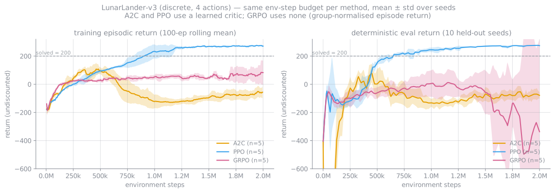
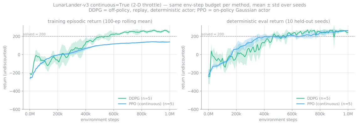
Protocol. After training, each seed's final policy is evaluated deterministically
(argmax for categorical, Gaussian mean, or $\mu(s)$ with no noise) on 50 fixed held-out reset seeds
(2,000,000,000–2,000,000,049) that are never used for training or checkpoint selection. "±" is the
standard deviation across the 5 seed means. "Solve rate" pools all 250 episodes. "Best-ckpt" re-evaluates
each seed's best.pt, chosen on a different 10-seed periodic eval, on the same 50
seeds.
| Config | Env | Budget | Final eval | Solve rate | Best-ckpt eval | Steps to first eval ≥ 200 | Wall-clock / seed | Env steps / s |
|---|---|---|---|---|---|---|---|---|
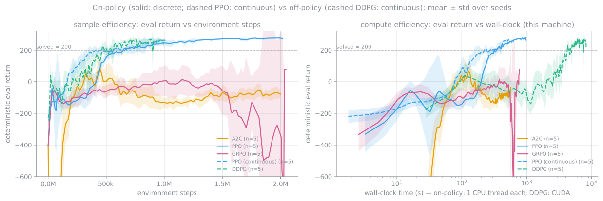
| PPO | discrete | 2.0M | 275.9 ± 2.5 | 99.6 % | 275.7 ± 2.6 | 612,762 (5/5) | 946 s | 2,134 |
| A2C | discrete | 2.0M | −64.7 ± 62.2 | 3.6 % | 122.7 ± 18.6 | never (0/5) | 549 s | 3,647 |
| GRPO | discrete | 2.0M | −388.9 ± 746.6 −16.7 ± 63.3 excl. seed 4 | 2.0 % | 51.0 ± 61.0 | never (0/5) | 743 s | 2,735 |
| PPO (continuous) | continuous | 1.0M | 265.0 ± 2.9 | 100 % | 265.2 ± 4.9 | 419,430 (5/5) | 511 s | 1,993 |
| DDPG | continuous | 1.0M | 249.1 ± 27.8 | 85.6 % | 270.5 ± 9.9 | 406,000 (5/5) | 8,249 s | 121 |
| SB3 PPO (reference only) | discrete | 2.0M | 274.0 ± 0.6 (3 seeds) | 98.7 % | — | 525,008 (3/3) | 1,708 s | 1,172 |
Wall-clock was measured with 13 jobs sharing the machine, and the on-policy jobs ran under nice -n 10, so
absolute steps/s are lower than a solo run would give. Only the ratios between methods are meaningful.
Evals ran every 25k steps for the on-policy methods and every 10k for DDPG. Each seed's training is
bit-reproducible on this machine: a first sweep that was stopped early and restarted produced identical
final evals for every seed that finished in both.
8.1 Learning progression, same starts
Every run saved a policy snapshot at each periodic evaluation. For the median seed by final eval, the snapshots at 0 / 2.5 / 10 / 25 / 50 / 100 % of the budget were flown deterministically from the same 20 held-out initial states (reset seeds 4,000,000,000 onward). DDPG has 5 stages because its first non-zero snapshot is at 50k = 5 %. Mean return / fraction landed, measured:
| Config (median seed) | 0 % | ~2.5–5 % | 10 % | 25 % | 50 % | 100 % |
|---|---|---|---|---|---|---|
| PPO (s4) | −603 / 0 % | −60 / 35 % | −138 / 5 % | 111 / 65 % | 215 / 90 % | 270 / 100 % |
| A2C (s0) | −345 / 0 % | −2,833 / 0 % | −230 / 0 % | −89 / 10 % | −18 / 25 % | −71 / 15 % |
| GRPO (s3) | −363 / 0 % | −183 / 0 % | −168 / 0 % | 31 / 50 % | 84 / 35 % | −25 / 0 % (100 % timeout) |
| PPO-cont. (s4) | −236 / 0 % | −109 / 0 % | −65 / 0 % | 71 / 45 % | 242 / 100 % | 261 / 100 % |
| DDPG (s3) | −110 / 0 % | — | −196 / 0 % | −101 / 10 % | 178 / 80 % | 261 / 100 % |
Each method page carries its own progression figure and video. All videos are 640×400 H.264 web encodes. 1920×1080 masters of every rollout and progression video exist for YouTube upload but are not deployed with the site.
9 · References
- Sutton & Barto, Reinforcement Learning: An Introduction, 2nd ed., 2018. MDPs, Bellman equations, §13 policy gradients.
- Sutton, McAllester, Singh, Mansour, Policy Gradient Methods for Reinforcement Learning with Function Approximation, NeurIPS 2000. Eq. (7).
- Williams, Simple Statistical Gradient-Following Algorithms for Connectionist RL (REINFORCE), Machine Learning 1992. The log-derivative estimator and baselines.
- Schulman, Moritz, Levine, Jordan, Abbeel, High-Dimensional Continuous Control Using Generalized Advantage Estimation, ICLR 2016. Eq. (12).
- Thomas, Bias in Natural Actor-Critic Algorithms, ICML 2014; Nota & Thomas, Is the Policy Gradient a Gradient?, AAMAS 2020. The dropped $\gamma^t$.
- Pardo, Tavakoli, Levdik, Kormushev, Time Limits in Reinforcement Learning, ICML 2018. §5.1.
- Ng, Harada, Russell, Policy Invariance under Reward Transformations, ICML 1999. Potential-based shaping, eq. (14)–(15).
- Towers et al., Gymnasium, 2024.
LunarLander-v3.
Continue with: On-policy vs off-policy · A2C · PPO · GRPO · DDPG · PPO & GRPO for LLMs · and the applied LLMs & SQL-GRPO track.