
DDPG — deep deterministic policy gradient
The three on-policy methods on this site sample an action from a distribution and push up the probability of the good ones. DDPG (Lillicrap et al., 2016) does something structurally different: the actor outputs one action, a learned critic $Q_w(s,a)$ says how good it is, and the actor follows the critic's gradient with respect to the action. That makes the method off-policy, so every transition goes into a replay buffer and is reused about 250 times. It also means the actor climbs whatever errors the critic has. This page derives the deterministic policy gradient, then derives and measures the over-estimation bias that follows from it.
Shared background (MDP, Bellman equations) is on the RL overview. The
on-policy/off-policy argument, including the deadly triad and data-reuse counts, is on
its own page and is not repeated here. DDPG runs only on
LunarLander-v3, continuous=True, so it is compared with PPO on the
same continuous environment, same 1M-step budget. Numbers marked measured are from 5 seeds on this machine.
1 · The deterministic policy-gradient theorem
Let the policy be a deterministic map $\mu_\theta : \mathcal S \to \mathcal A$, here a 400×300 ReLU MLP with a tanh output so that $\mu_\theta(s)\in[-1,1]^2$. Its value functions satisfy $V^{\mu}(s) = Q^{\mu}(s, \mu_\theta(s))$ and the Bellman equation
$$ Q^{\mu}(s,a) = r(s,a) + \gamma \int P(s'\mid s,a)\, V^{\mu}(s')\, ds' \tag{1} $$The objective is $J(\theta) = \int \rho_0(s)\, V^{\mu}(s)\, ds$. Differentiate $V^\mu(s) = Q^\mu(s,\mu_\theta(s))$. $\theta$ enters in two places: through the action $a = \mu_\theta(s)$ chosen now, and through the policy followed afterwards, which is hidden inside $Q^\mu$. By the chain rule,
$$ \nabla_\theta V^{\mu}(s) = \nabla_\theta\mu_\theta(s)\,\nabla_a Q^{\mu}(s,a)\big|_{a=\mu_\theta(s)} \;+\; \nabla_\theta Q^{\mu}(s,a)\big|_{a=\mu_\theta(s)} \tag{2} $$$\nabla_\theta\mu_\theta(s)$ is the $\dim\theta \times \dim\mathcal A$ Jacobian of the actor. The second term comes from differentiating (1) with $a$ held fixed. $r$ and $P$ do not depend on $\theta$, so $\nabla_\theta Q^\mu(s,a) = \gamma\int P(s'\mid s,a)\,\nabla_\theta V^\mu(s')\,ds'$. Substituting this back into (2) gives a recursion of the same form one step later. Unrolling it, and writing $p(s\to s', t, \mu)$ for the density of reaching $s'$ from $s$ after $t$ steps under $\mu$:
$$ \nabla_\theta V^{\mu}(s) = \sum_{t=0}^{\infty}\gamma^t \int p(s\to s',t,\mu)\; \nabla_\theta\mu_\theta(s')\,\nabla_a Q^{\mu}(s',a)\big|_{a=\mu_\theta(s')}\, ds' \tag{3} $$Integrating over $\rho_0$ and collecting the discounted visitation into $\rho^\mu(s') = \int\rho_0(s)\sum_t\gamma^t p(s\to s',t,\mu)\,ds$ gives the deterministic policy-gradient theorem (Silver et al., 2014):
$$ \nabla_\theta J(\theta) = \mathbb{E}_{s\sim\rho^{\mu}}\Big[\nabla_\theta\mu_\theta(s)\; \nabla_a Q^{\mu}(s,a)\big|_{a=\mu_\theta(s)}\Big] \tag{4} $$(The exchange of derivative and integral, and the convergence of the series, need regularity conditions on $P$, $r$ and $\mu$; Silver et al. state them in their Appendix A.) Read (4) as a chain rule: the critic says which way to move the action to increase $Q$, and the actor's Jacobian translates that into a direction in weight space. Compare the stochastic theorem (overview 7). There is no expectation over actions, and so no $\nabla\log\pi$ score function and no sampling noise from the action. That is the method's strength: lower-variance gradients in continuous action spaces. It is also its weakness, because the whole gradient now comes from $\nabla_a Q$, which must be learned.
In practice $Q^\mu$ is replaced by the critic $Q_w$, and the actor minimises $\mathcal L_\mu(\theta) = -\mathbb{E}_{s\sim\mathcal D}\big[Q_w(s, \mu_\theta(s))\big]$. Autograd computes exactly (4) through the composition, with $w$ held fixed:
2 · The critic: TD target, target networks, replay
2.1 TD target
The critic regresses onto a one-step bootstrapped target built from (1). For a minibatch $\{(s_i,a_i,r_i,s'_i,d_i)\}$ of 256 transitions drawn from the buffer $\mathcal D$, with $d_i = 1$ only for a true terminal:
$$ y_i = r_i + \gamma\,(1-d_i)\, Q_{w'}\big(s'_i,\ \mu_{\theta'}(s'_i)\big), \qquad \mathcal L_Q(w) = \frac{1}{256}\sum_i\big(Q_w(s_i,a_i) - y_i\big)^2 \tag{5} $$$\gamma = 0.99$. A time-limit truncation is stored with $d = 0$, so it still bootstraps (overview §5.1). $Q_{w'}$ and $\mu_{\theta'}$ are the target networks.
2.2 Target networks and Polyak averaging
If $y$ were computed with $Q_w$ itself, every gradient step on $w$ would move the target it is chasing, and with function approximation this feedback can diverge. DDPG keeps slow copies and updates them by Polyak averaging after every gradient step:
$$ w' \leftarrow (1-\tau)\,w' + \tau\,w, \qquad \theta' \leftarrow (1-\tau)\,\theta' + \tau\,\theta, \qquad \tau = 0.005 \tag{6} $$So $w'$ is an exponential moving average of $w$ with a time constant of $1/\tau = 200$ updates. The target lags behind the critic it is training, which turns a moving-target problem into something close to supervised regression on a slowly drifting target. It damps the feedback loop of the deadly triad but does not remove it.
2.3 Replay buffer
Every transition goes into a 1,000,000-slot ring buffer (s [1e6, 8], a [1e6, 2], r [1e6], s' [1e6, 8],
term [1e6]), and each update samples 256 uniformly. That serves two purposes. It breaks the strong temporal
correlation of consecutive 50 Hz states, so minibatches look closer to i.i.d. And it reuses data: after a
10,000-step uniform-random warm-up, 990,000 updates × 256 samples means each stored transition is drawn
about 250 times on average.
3 · Why off-policy learning is valid here
The data in $\mathcal D$ was generated by a mixture of old, noisy behaviour policies $\beta$, not by the current $\mu_\theta$. There are two places where that could matter, and neither needs an importance ratio:
- The critic target (5). Equation (1) for a deterministic policy has no expectation over actions at the next state: $\mu_{\theta'}(s')$ is evaluated directly. The only expectation left is over $s' \sim P(\cdot\mid s,a)$, and every stored $(s,a,r,s')$ is a valid sample of it whoever chose $a$. A stochastic target policy would need $\mathbb{E}_{a'\sim\pi}$, which you can still evaluate by sampling from $\pi$, so Q-learning-style critics are off-policy either way. What a deterministic policy removes is the actor's need for a ratio.
- The actor gradient (4). The stochastic policy gradient averages $\nabla\log\pi(a\mid s)$ over actions drawn from $\pi$ itself, so reusing old actions requires reweighting by $\pi/\beta$. (4) has no integral over actions at all: it evaluates $\nabla_a Q$ at $a = \mu_\theta(s)$, which we can compute for any stored $s$. Silver et al. (2014) write the off-policy version as $\nabla_\theta J_\beta \approx \mathbb{E}_{s\sim\rho^\beta}[\nabla_\theta\mu_\theta(s)\,\nabla_a Q^\mu(s,a)|_{a=\mu_\theta(s)}]$.
4 · Exploration: Gaussian, not Ornstein–Uhlenbeck
A deterministic actor never explores on its own. The behaviour policy adds noise:
$$ a_t = \operatorname{clip}\big(\mu_\theta(s_t) + \sigma\,\xi_t,\ -1,\ 1\big), \qquad \xi_t\sim\mathcal N(0, I_2),\; \sigma = 0.1 \tag{7} $$
The 2016 paper used temporally correlated Ornstein–Uhlenbeck noise, motivated by physical systems with
inertia, where white noise averages out before it moves anything. ddpg.py uses uncorrelated
Gaussian noise instead, following Fujimoto et al. (2018, §6.1, "OurDDPG"), who found it matches OU on
MuJoCo. It has one fewer hyper-parameter (the mean-reversion rate) and no hidden state to reset at episode
boundaries. LunarLander's engines also respond instantly at 50 Hz. The first 10,000 steps use uniformly
random actions to seed the buffer before any update.
5 · Over-estimation, the centrepiece
5.1 Why maximising through a learned Q biases it upward
Write the critic as truth plus error, $Q_w(s,a) = Q^\mu(s,a) + \varepsilon(s,a)$, and suppose the error is unbiased: $\mathbb{E}[\varepsilon(s,a)] = 0$ for every fixed $(s,a)$. Let $a^* = \arg\max_a Q^\mu(s,a)$ be the truly best action, and $\hat a = \arg\max_a Q_w(s,a)$ the action the actor is driven toward by (4). Because $\hat a$ maximises $Q_w$,
$$ Q_w(s,\hat a) \;\ge\; Q_w(s,a^*) = Q^\mu(s,a^*) + \varepsilon(s,a^*) \tag{8} $$Take expectations over the critic's error. The right-hand side has expectation $Q^\mu(s,a^*) = \max_a Q^\mu(s,a)$, because $a^*$ is fixed and does not depend on $\varepsilon$. So
$$ \mathbb{E}_\varepsilon\Big[\max_a Q_w(s,a)\Big] \;\ge\; \max_a Q^\mu(s,a) \tag{9} $$with strict inequality whenever the errors at different actions are not perfectly correlated: the max preferentially picks actions whose error happens to be positive. This is Jensen's inequality for the convex $\max$, and the argument is Thrun & Schwartz's (1993) for tabular Q-learning. Fujimoto et al. (2018) showed it carries over to a deterministic actor that does gradient ascent on $Q_w$, because the actor is an approximate argmax.
Bootstrapping compounds it. The target (5) evaluates $Q_{w'}$ at $\mu_{\theta'}(s')$, an action chosen to make $Q$ large, so each target inherits the upward bias of the next state. If the per-step bias were a constant $b$, unrolling (5) would give a steady-state bias of about
$$ \text{bias}_\infty \approx \sum_{k\ge 0}\gamma^k\, b = \frac{b}{1-\gamma} = 100\,b \quad (\gamma = 0.99) \tag{10} $$So a small per-step error is amplified by up to the effective horizon. Target networks slow the propagation but do not change the fixed point.
5.2 Measured: the Q-versus-return gap
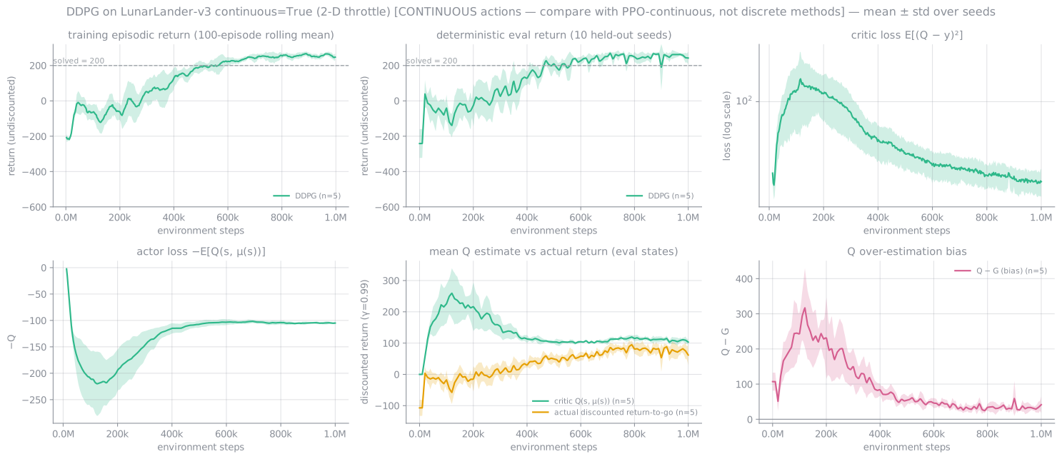
At every periodic evaluation (every 10k steps), ddpg.py flies 10 deterministic episodes, computes the
critic's $Q_w(s_t, \mu(s_t))$ on every visited state, and compares it with the actual discounted return-to-go
$G_t = \sum_k \gamma^k r_{t+k}$ from that state in the same episode:
| seed 0 | seed 1 | seed 2 | seed 3 | seed 4 | |
|---|---|---|---|---|---|
| Peak bias $\overline{Q_w - G}$ | +459 | +495 | +320 | +358 | +250 |
| Peak predicted $\bar Q_w$ / true $\bar G$ at that eval | 367 / −14 | 373 / −122 | 240 / −79 | 293 / −46 | 205 / 26 |
| Bias at the final eval | +23.3 | +23.9 | +67.5 | +20.2 | +72.2 |
| Bias, median of last 20 evals | +33.3 | +26.0 | +39.2 | +27.7 | +17.5 |
| Critic loss: peak → final | 222 → 24.6 | 314 → 24.8 | 117 → 29.5 | 178 → 27.1 | 67 → 13.2 |
5.3 What you would do next: TD3's three fixes
Fujimoto et al. (2018) designed TD3 against exactly this failure. All three changes are small edits to (5) and the update loop:
- Clipped double-Q. Train two critics $Q_{w_1}, Q_{w_2}$ and use the smaller in the target: $y = r + \gamma(1-d)\min_{j=1,2} Q_{w'_j}(s', \tilde a')$. The min of two noisy estimates is biased downward, which counteracts (9). Under-estimation is the safer error because the actor does not seek it out.
- Target policy smoothing. $\tilde a' = \operatorname{clip}\big(\mu_{\theta'}(s') + \operatorname{clip}(\epsilon, -c, c), -1, 1\big)$, $\epsilon\sim\mathcal N(0,\tilde\sigma^2)$. Averaging the target over a small neighbourhood of actions stops the actor exploiting narrow spikes in $Q_w$.
- Delayed policy updates. Update the actor (and the targets) once every 2 critic updates, so the actor follows a critic whose error has had time to fall.
None of these was run here. The brief was DDPG as published (with the TD3 authors' re-tuned settings), and the measured bias above is what motivates them. SAC (Haarnoja et al., 2018) uses the same clipped double-Q plus an entropy-regularised stochastic actor.
6 · Implementation: hyper-parameters, training, inference
| Parameter | Value | Reason |
|---|---|---|
| Actor $\mu_\theta$ | 8 → 400 → 300 → 2 → tanh, ReLU, PyTorch default init, 124,502 params | TD3/OurDDPG reference |
| Critic $Q_w$ | concat(s, a) = 10 → 400 → 300 → 1, ReLU, 125,001 params | Action enters at the input (TD3 style) |
| Actor / critic lr | 1e-3 / 1e-3, Adam | OurDDPG. The 2016 paper's 1e-4 / 1e-3 is weaker |
| Batch, buffer, warm-up | 256, 1,000,000, 10,000 uniform steps | OurDDPG |
| $\gamma$, $\tau$ | 0.99, 0.005 | OurDDPG |
| Critic L2 | none | OurDDPG removed the paper's 1e-2 |
| Exploration | Gaussian $\sigma = 0.1$ | §4 |
| Updates per env step | 1 | OurDDPG |
| Device | CUDA | Measured: 388 vs 115 updates/s on 1 CPU thread (182 on 4) for these nets at batch 256 |
The networks are about 25× larger than the on-policy 2×64 nets, following the reference architecture, and each has a target copy, so four 125k-parameter networks are held during training. Only the actor is deployed: one forward pass costs 138 µs on one CPU thread at batch 1, measured under load.
6.1 Training loop, step by step
Read the listing against the on-policy ones. There is no rollout, no advantage, no ratio and no discard. Each environment step is followed by exactly one critic step and one actor step, on data that can be up to a million steps old. Step (b) is the only place the reward enters, and step (c) is the only place the actor learns, entirely through $\nabla_a Q_w$. Any error in $Q_w$ goes straight into the actor, which is §5 in one line.
6.2 Inference
Training needs four 125k-parameter networks and a million-row buffer. Deployment needs one of the networks. The controller you ship is $\mu_\theta$ with the exploration noise of (7) removed, so it is a different policy from the one that collected most of the buffer. That is harmless for DDPG's learning rule, which never needed the behaviour policy's probabilities.
7 · Results against PPO-continuous (measured)
| Config, continuous env, 1M steps | Final eval (50 eps) | Solve rate | Best-ckpt eval | Steps to first eval ≥ 200 | Wall-clock / seed | Env steps / s |
|---|---|---|---|---|---|---|
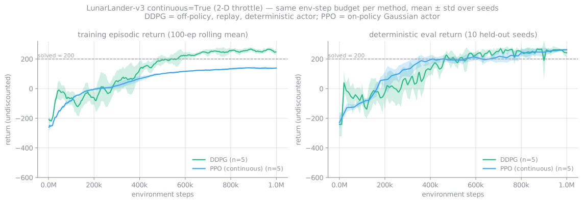
| DDPG | 249.1 ± 27.8 | 85.6 % | 270.5 ± 9.9 | 406,000 (5/5) | 8,249 s | 121 |
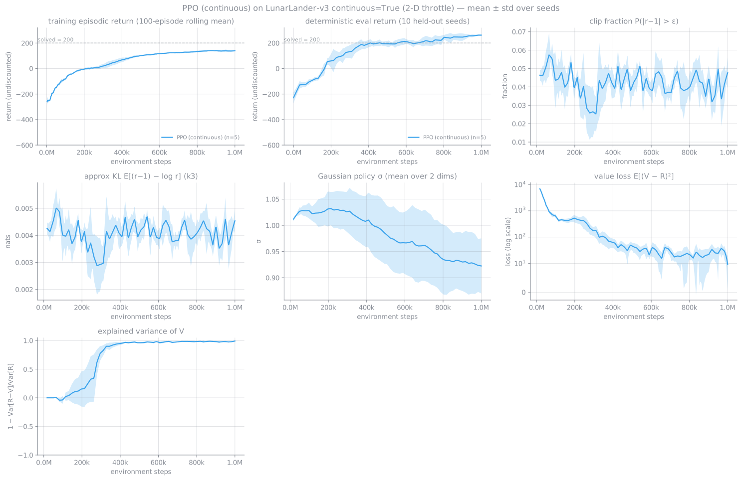
| PPO-continuous | 265.0 ± 2.9 | 100 % | 265.2 ± 4.9 | 419,430 (5/5) | 511 s | 1,993 |
Per-seed DDPG final / best-checkpoint: 273.9 / 280.7, 273.8 / 261.1, 228.5 / 262.2, 264.4 / 264.4, 204.6 / 284.3. First eval ≥ 200 per seed: 460k, 350k, 410k, 540k, 270k. All are deterministic $\mu(s)$, on the 50 held-out final-eval seeds, measured on this machine with 13 jobs sharing it.
1. Not more sample-efficient. The first eval ≥ 200 came at 406k steps for DDPG and 419k for PPO-continuous: a tie within seed spread, despite DDPG reusing each transition about 250 times.
2. 16× the wall-clock. 8,249 s vs 511 s per seed. DDPG takes 1 gradient step per env step on 256 samples through about 125k-parameter nets, and its loop is sequential. PPO takes 1/16 of a step per env step through about 5k-parameter nets, and its environment collection is embarrassingly parallel.
3. Higher peaks, worse finish. DDPG's best checkpoints (270.5 ± 9.9) slightly beat PPO-continuous, but seeds 2 and 4 degraded late, to 228.5 and 204.6 against best checkpoints of 262.2 and 284.3. The 50-episode solve rate is 85.6 % for final policies and 96.4 % for best checkpoints. That gap is why DDPG results are usually reported at the best checkpoint, and the persistent positive Q bias of §5.2 is the most likely source of the late drift.
7.1 Both controllers, flown
best.pt, deterministic $\mu(s)$ with no exploration noise, recorded on this machine.
Flown on a pool of 24 held-out video seeds (3,000,000,000 onward): 23 / 24 score ≥ 200 (23 landed, 1 timeout).
Fewer than 15 % failed, so the video shows 4 successful episodes: 251, 274, 288 and 293, all landed.
640×400 H.264, 18.4 s.
best.pt, deterministic (Gaussian mean), recorded on this machine.
Same 24-seed video pool: 24 / 24 score ≥ 200, all landed. Shown: 235, 264, 271 and 284. 640×400 H.264, 25.8 s.
1920×1080 masters of both videos and of the progression videos exist for YouTube upload but are not deployed with the site.
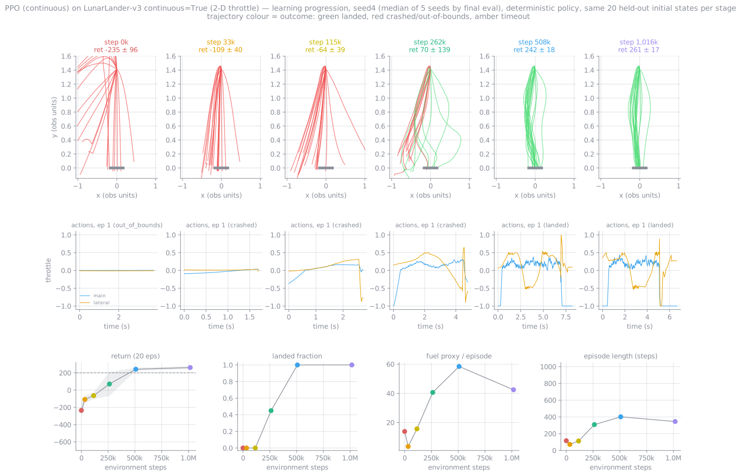
7.2 Learning progression from the same starts
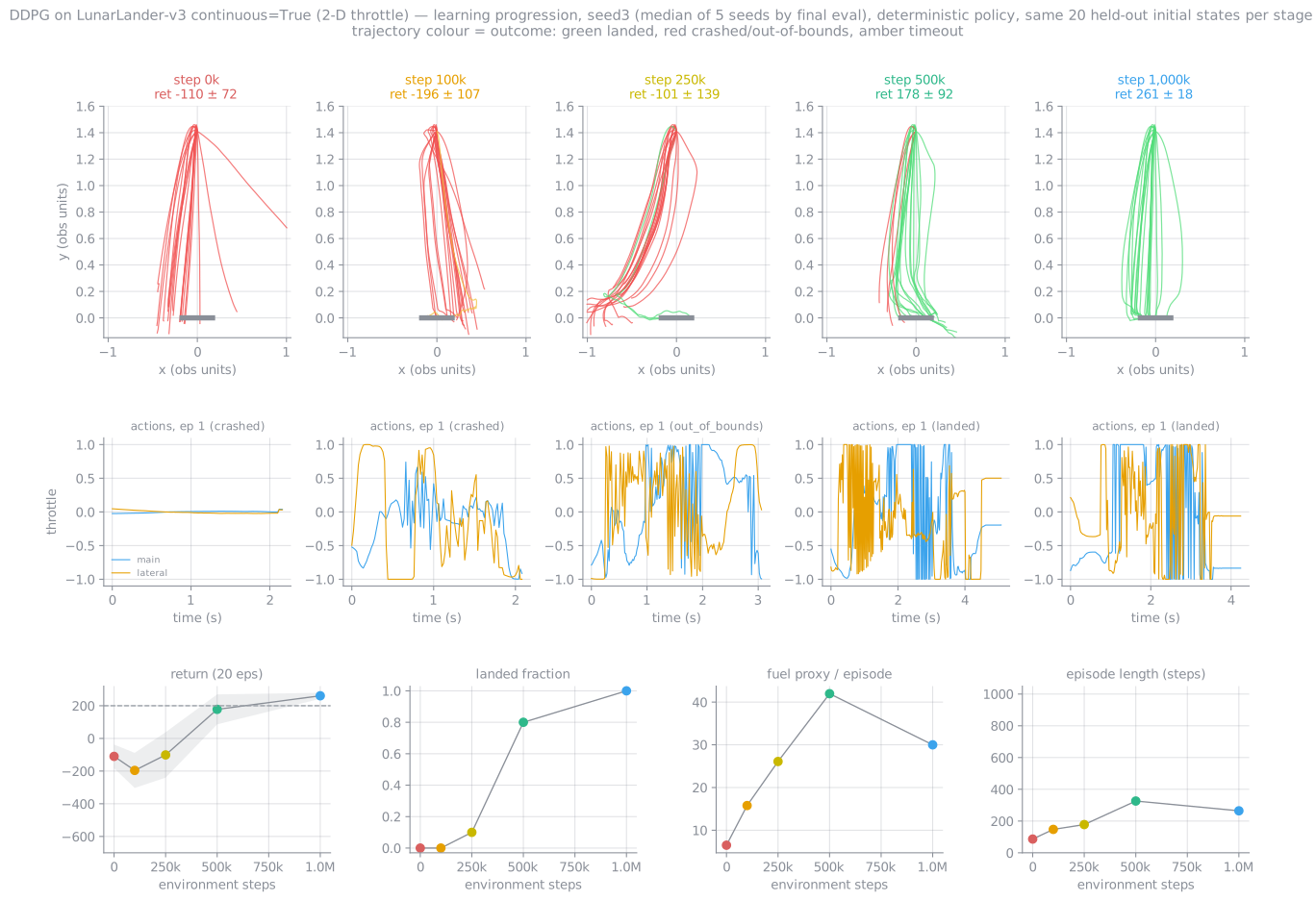
Median seed by final eval, deterministic, the same 20 held-out initial states at each stage. DDPG snapshots every 50k steps, so it has 5 stages (0, 10, 25, 50, 100 %) rather than 6. Mean return / fraction landed, measured:
| Median seed | 0 % | 2.5 % | 10 % | 25 % | 50 % | 100 % |
|---|---|---|---|---|---|---|
| DDPG (s3) | −110 / 0 % | — | −196 / 0 % | −101 / 10 % | 178 / 80 % | 261 / 100 % |
| PPO-continuous (s4) | −236 / 0 % | −109 / 0 % | −65 / 0 % | 71 / 45 % | 242 / 100 % | 261 / 100 % |
The two curves have nearly the same shape. Neither shows the "competent within a few percent of the budget" behaviour often credited to off-policy methods. DDPG is competent from about 50 % of the budget, which matches when its Q bias has shrunk from its peak.
8 · Honest limitations
- Structural over-estimation (§5), measured on every seed and never fully gone. Use TD3 or SAC in practice.
- Late instability. 2 of 5 seeds lost 34–80 points from their best checkpoint. Results depend on checkpoint selection.
- Continuous actions only. (4) needs $\nabla_a Q$, so DDPG cannot be compared directly with the discrete A2C/PPO/GRPO runs.
- Compute-hungry and sequential. 16× PPO's wall-clock here, with one env and one update per step. It parallelises poorly without distributed replay.
- Hyper-parameter sensitivity. $\tau$, noise scale, learning rates, buffer size and warm-up all matter, and none was tuned. These are the TD3 authors' re-tuned values.
9 · References
- Silver, Lever, Heess, Degris, Wierstra, Riedmiller, Deterministic Policy Gradient Algorithms, ICML 2014. Eq. (4), Appendix A.
- Lillicrap, Hunt, Pritzel, Heess, Erez, Tassa, Silver, Wierstra, Continuous Control with Deep Reinforcement Learning, ICLR 2016. DDPG.
- Fujimoto, van Hoof, Meger, Addressing Function Approximation Error in Actor-Critic Methods, ICML 2018. TD3 and the "OurDDPG" settings.
- Thrun & Schwartz, Issues in Using Function Approximation for Reinforcement Learning, 1993. Eq. (9).
- van Hasselt, Double Q-learning, NeurIPS 2010. The idea behind clipped double-Q.
- Degris, White, Sutton, Off-Policy Actor-Critic, ICML 2012. The state-distribution approximation.
- Haarnoja, Zhou, Abbeel, Levine, Soft Actor-Critic, ICML 2018.
- Mnih et al., Human-level control through deep RL (DQN), Nature 2015. Replay and target networks.
Related: On-policy vs off-policy · PPO · back to the RL overview