
Architecture modules
A dictionary for the "modules" column of the comparison table. Each entry answers three questions: what the block computes, what problem it was introduced to solve, and what it costs. Modules are grouped by where they sit in the pipeline — image to tokens, tokens to the language model, attention mechanics, and pixel generation.
Symbols used on this page are defined in the Nomenclature → learning.
1 · From image to tokens
1.1 Vision transformer (ViT)
Cut the image into a grid of non-overlapping patches, flatten each, project it linearly, add a position embedding, and run the sequence through a standard transformer encoder. For a $H\times W$ image with patch size $P$:
$$ N = \frac{HW}{P^2}, \qquad \mathbf z_0 = \big[\mathbf x_{\text{cls}};\, E\mathbf p_1;\, \dots;\, E\mathbf p_N\big] + \mathbf E_{\text{pos}} $$The numbers matter for cost, because self-attention is quadratic in $N$. At 224 px with $P=14$ you get $N=256$; at 336 px, $N=576$; at 1024 px, $N=5{,}329$ — a 20× token increase and a 400× attention cost over the 224 px case. This single relationship explains most of the resolution engineering in the model table.
| Variant | Patch | Tokens at native res | Where it shows up |
|---|---|---|---|
| ViT-B/32 | 32 | 49 @ 224 px | Original CLIP, cheap retrieval |
| ViT-L/14 | 14 | 256 @ 224, 576 @ 336 | CLIP-L — the most reused vision tower |
| ViT-H/14, g/14, G/14 | 14 | 256+ | OpenCLIP, EVA, Llama 3.2 Vision |
| SigLIP-So400m | 14/16 | varies | PaliGemma, Idefics, many 2024–25 models |
1.2 Swin transformer — hierarchical windowed attention
A plain ViT has one resolution and global attention at every layer. Swin instead computes attention inside local windows of $M\times M$ patches and merges patches between stages, producing a feature pyramid like a CNN. The cost difference is the point:
$$ \Omega(\text{global}) = 4ND^2 + 2N^2D, \qquad \Omega(\text{window}) = 4ND^2 + 2M^2ND $$The $N^2$ term becomes $M^2 N$ — linear in the number of patches. Pure windowing would prevent information crossing window boundaries, so alternate layers shift the window grid by $M/2$, which reconnects neighbours without giving up linearity.
1.3 Feature pyramid network (FPN)
Small objects need high-resolution features; recognising what they are needs deep, semantic features. In a plain CNN those are at opposite ends of the network. An FPN builds a top-down path that carries semantics back down to high resolution, fusing by elementwise addition after a $1\times1$ projection:
$$ P_l = \operatorname{Conv}_{3\times3}\Big( \operatorname{Conv}_{1\times1}(C_l) + \operatorname{Upsample}(P_{l+1})\Big) $$Each level then predicts at its own scale. FPNs are ubiquitous in detectors and in the BEV stacks on the perception pages, but they are largely absent from VLMs — another consequence of the "one flat sequence" requirement. Where a VLM needs multi-scale detail it gets it by tiling the input instead, which is a cruder but architecture-free solution.
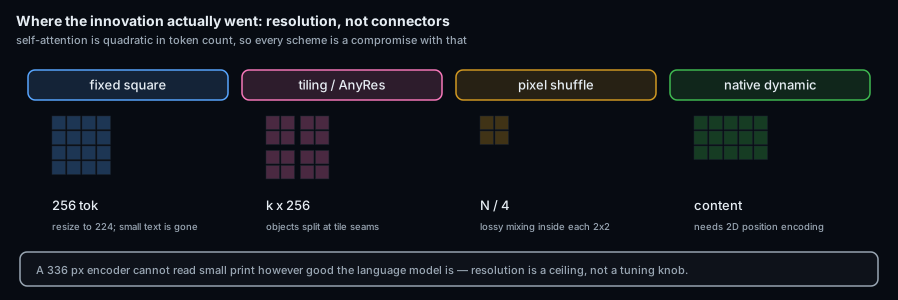
1.4 Resolution strategies — where the real innovation went
| Strategy | Mechanism | Cost | Weakness |
|---|---|---|---|
| Fixed square | Resize to 224/336, accept the loss | Cheapest | Small text is unreadable; aspect ratio destroyed |
| AnyRes / tiling LLaVA-NeXT, InternVL |
Cut into fixed tiles, encode each, plus a downscaled global view | Linear in tiles | Objects straddling a tile boundary are split; tokens explode |
| Pixel shuffle InternVL |
Trade channels for space: fold a $2\times2$ neighbourhood into the channel dim | ¼ the tokens | Lossy spatial mixing inside each group |
| Native dynamic Qwen2-VL, Pixtral |
Variable token count with 2D position encodings; no resizing | Scales with content | Needs 2D-aware position encoding and careful batching |
| No encoder Fuyu |
Project raw patches straight into the decoder | Simplest code path | Forfeits all contrastive pretraining; needs far more data |
2 · Contrastive objectives
2.1 CLIP and the InfoNCE loss
Two encoders, one shared space. In a batch of $B$ pairs, the matched pair is the positive and the other $B-1$ are negatives; the loss is symmetric cross-entropy over the similarity matrix, with a learned temperature $\tau$:
$$ \mathcal L = -\frac{1}{2B}\sum_{i=1}^{B}\left[ \log\frac{e^{s_{ii}/\tau}}{\sum_j e^{s_{ij}/\tau}} + \log\frac{e^{s_{ii}/\tau}}{\sum_j e^{s_{ji}/\tau}}\right], \qquad s_{ij} = \frac{\mathbf u_i^{\mathsf T}\mathbf v_j}{\|\mathbf u_i\|\,\|\mathbf v_j\|} $$Two consequences are worth stating plainly. First, quality depends on batch size, because the batch is the negative set — CLIP used 32,768. Second, the softmax is over the whole batch, so distributed training requires an all-gather of every embedding on every step.
2.2 SigLIP and the pairwise sigmoid loss
Replace the softmax with an independent binary classification on every pair:
$$ \mathcal L = \frac{1}{B}\sum_{i=1}^{B}\sum_{j=1}^{B} \log\!\Big(1 + e^{\,z_{ij}\,(-t\,s_{ij} + b)}\Big), \qquad z_{ij} = \begin{cases} +1 & i = j \\ -1 & i \ne j\end{cases} $$with learned temperature $t$ and a learned bias $b$. The bias exists because the pair matrix is massively imbalanced — $B$ positives against $B^2 - B$ negatives — and $b$ absorbs that prior.
| InfoNCE (CLIP) | Sigmoid (SigLIP) | |
|---|---|---|
| Normalisation | Global softmax over the batch | None — per-pair |
| Distributed cost | All-gather every embedding | Local chunks suffice |
| Small-batch behaviour | Degrades sharply | Still works |
| Large-batch behaviour | Keeps improving | Saturates earlier (~32K) |
3 · Connectors — vision to language
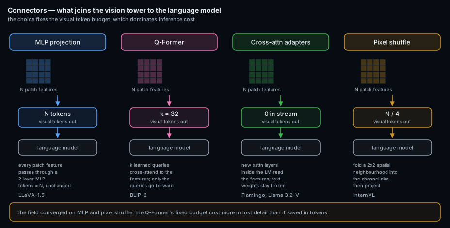
The vision encoder emits $N$ feature vectors of dimension $D_v$; the language model consumes tokens of dimension $D_t$. The connector bridges that, and in doing so fixes the visual token budget, which is the dominant term in inference cost.
| Connector | Computation | Visual tokens | Trade |
|---|---|---|---|
| Linear | $\mathbf t_i = W\mathbf f_i$ | $=N$ | Lossless but expensive; grows with resolution |
| MLP (2 layers) | $W_2\,\sigma(W_1\mathbf f_i)$ | $=N$ | The current default. More capacity, same token count |
| Q-Former | $k$ learned queries cross-attend to the features | $=k$, typically 32 | Fixed cost at any resolution — but an information bottleneck |
| Perceiver resampler | Same idea, lighter, no self-supervised pretraining | $=k$ | As above |
| Cross-attention adapters | New xattn layers inside the LM read the features | 0 in the text stream | Text weights can stay frozen; costs new parameters per layer |
| Pixel shuffle | Fold $2\times2$ spatial into channels, then MLP | $=N/4$ | Cheap and surprisingly effective |
3.1 The Q-Former, and why it fell out of favour
BLIP-2's Q-Former is a small transformer holding $k=32$ learned query vectors. The queries self-attend, cross-attend to the frozen image features, and the 32 outputs become the visual tokens. It was trained in two stages with three objectives at once — image-text contrastive, image-text matching, and image-grounded text generation — with different attention masks per objective.
It is an elegant design and it solved a real problem: 32 tokens is a fixed, small cost. But compressing a 576-token image into 32 vectors discards spatial detail irreversibly, and when the field moved to documents and dense text that loss became the binding constraint. A plain MLP keeping all 576 tokens beat it, and the complexity was abandoned.
4 · Attention mechanics
4.1 Flash attention
Flash attention computes exactly the same function as standard attention. It is not an approximation — it is an IO-aware implementation, and the distinction matters because it means there is never an accuracy reason not to use it.
Standard attention materialises the $N\times N$ matrix $QK^{\mathsf T}$ in GPU high-bandwidth memory, costing $O(N^2)$ memory traffic. Flash attention tiles $Q$, $K$ and $V$ into blocks that fit in on-chip SRAM and accumulates the softmax with a running maximum and running denominator, so the big matrix is never written out:
$$ m^{(j)} = \max\!\big(m^{(j-1)},\, \tilde m^{(j)}\big), \qquad \ell^{(j)} = e^{\,m^{(j-1)} - m^{(j)}}\ell^{(j-1)} + e^{\,\tilde m^{(j)} - m^{(j)}}\tilde\ell^{(j)} $$Memory falls from $O(N^2)$ to $O(N)$, which is what makes long-context and high-resolution models trainable at all. In the backward pass the attention matrix is recomputed from the saved statistics rather than stored — trading arithmetic, which is cheap, for memory traffic, which is not.
4.2 Attention variants you will see in the table
| Variant | Idea | Why |
|---|---|---|
| MHA → MQA → GQA | Share key/value heads across query heads | Shrinks the KV cache, which dominates memory at inference |
| Window attention | Attend only within a local window | Linear in sequence length; used in Swin and Qwen2.5-VL's encoder |
| Deformable attention | Learn a few sampling offsets per query | Sparse multi-scale attention — see RF-DETR |
| RoPE / M-RoPE / RoPE-2D | Rotate queries and keys by position-dependent angles | Relative positions, extrapolates; the multimodal variants encode (time, height, width) separately |
| Prefix-LM masking | Image and prompt tokens attend bidirectionally; only the answer is causal | The image is not a sequence, so forcing causality over it wastes capacity |
5 · Generation — VAEs, diffusion and flows
The maths of latent diffusion is derived in detail on the Stable Diffusion page. This section covers only what that page does not: the autoencoder's role, and the newer transformer and flow formulations.
5.1 The VAE, and what "latent" buys
Diffusion in pixel space is wasteful — most pixels are perceptually redundant. A VAE compresses by a factor of 8 spatially before any diffusion happens:
$$ \mathbf x \in \mathbb R^{3\times512\times512} \;\xrightarrow{\ \mathcal E\ }\; \mathbf z \in \mathbb R^{4\times64\times64} \qquad \text{a } 48\times \text{ reduction in elements} $$It is trained with a reconstruction term, a perceptual (LPIPS) term, a patch-adversarial term and a deliberately weak KL penalty. The KL weight is small on purpose: a strongly regularised latent would be smooth and well-behaved for sampling but would have thrown away the high-frequency detail the diffusion model needs. Newer models increase the channel count (SD3 uses 16) precisely because 4 channels were found to be a fidelity ceiling.
5.2 DiT, MMDiT and rectified flow
| Module | What changed | Why it matters |
|---|---|---|
| DiT | Replace the UNet with a transformer over latent patches; condition by modulating LayerNorm (adaLN-Zero) | Scales with parameters the way transformers do, unlike the UNet |
| MMDiT SD3 |
Separate weights for image and text streams, but attention is computed jointly | The two modalities have different statistics; sharing one projection handicaps both |
| Rectified flow | Train on straight interpolation $\mathbf z_t = (1-t)\mathbf x_0 + t\boldsymbol\epsilon$ and regress the constant velocity | A straight ODE path integrates accurately in few steps — this is the main reason modern samplers need 20 steps instead of 1,000 |
| Flow matching | The general framework rectified flow is one instance of | Unifies diffusion and continuous normalising flows; simpler objective |
The second is a straight line between data and noise, and its target velocity $\boldsymbol\epsilon - \mathbf x_0$ is constant along the path. That is the whole trick: curvature in the probability-flow path is what forces many small integration steps, so removing the curvature removes the steps.
5.3 Text conditioning, and a result that surprised people
| Encoder | Used by | Property |
|---|---|---|
| CLIP text | SD1.5, SDXL | Image-aligned but 77 tokens and trained on short alt-text; weak on long prompts |
| T5-XXL | Imagen, SD3, FLUX | Never saw an image, yet gives better prompt fidelity and spelling |
| Both | SD3, FLUX | CLIP for global alignment, T5 for compositional detail |
6 · Training stages
Nearly every model in the table follows the same three-stage recipe, and knowing which stage a claim comes from prevents a lot of confusion.
| Stage | What trains | Data | Purpose |
|---|---|---|---|
| 1 · Alignment | Connector only; both towers frozen | ~0.5–5M caption pairs | Teach the projection to speak the LM's embedding dialect without disturbing either tower |
| 2 · Pretraining | Connector + LM, sometimes the vision tower | 10M–10B interleaved documents | Build real visual knowledge |
| 3 · Instruction tuning | LM, usually with LoRA | ~100K–5M curated conversations | Make it answer the question asked, in the format asked |
| 4 · Preference (optional) | LM, via DPO/RLHF | Preference pairs | Reduce hallucination, improve helpfulness |
7 · References
The figures on this page are original redrawings in the site's palette, not reproductions — the architectures are credited to the papers below. Where a blog post is the clearest explanation of something, it is cited as such.
7.1 Backbones and attention
- Dosovitskiy et al., An Image is Worth 16x16 Words (ViT, ICLR 2021).
- Liu et al., Swin Transformer (ICCV 2021) — the windowed-attention cost argument in §1.2 follows their analysis.
- Lin et al., Feature Pyramid Networks (CVPR 2017).
- Dao et al., FlashAttention (NeurIPS 2022) and FlashAttention-2 (2023).
- Su et al., RoFormer (RoPE, 2021); Shazeer, Fast Transformer Decoding (MQA, 2019); Ainslie et al., GQA (2023).
7.2 Connectors and generation
- Jaegle et al., Perceiver IO (2021) — the resampler idea.
- Peebles and Xie, Scalable Diffusion Models with Transformers (DiT, ICCV 2023) — source of adaLN-Zero.
- Lipman et al., Flow Matching for Generative Modeling (ICLR 2023); Liu et al., Rectified Flow (2022).
- Saharia et al., Photorealistic Text-to-Image Diffusion Models with Deep Language Understanding (Imagen, 2022) — the T5-beats-CLIP result in §5.3.
Related: Model comparison table · Visual question answering · Image editing · Stable Diffusion · DINOv2 · DNN optimizers