
IMUs — what you can buy, and what the numbers mean
An IMU is three gyros and three accelerometers in a box, and its price spans four orders of magnitude for the same nominal function. What you are actually buying is how slowly the errors grow. This page maps the market by grade, gives representative parts with representative numbers, and — most importantly — connects each datasheet line to the term it becomes in your navigation error budget.
Symbols used on this page are defined in the Nomenclature → inertial navigation.
Indicative public-datasheet values for orientation, not procurement. Theory and the error model itself are on the IMU & inertial navigation page.
The five numbers that decide everything
| Spec | Units | What it does to your solution |
|---|---|---|
| Angle random walk (ARW) | °/√hr | White gyro noise. Attitude error grows as $\sigma\sqrt t$ — dominates in the first seconds after a fix. |
| Bias instability | °/hr | The Allan-variance floor. An uncorrected bias $b$ tilts the gravity vector and gives position error $\propto \tfrac16 g\,b\,t^3$. |
| Turn-on repeatability | °/hr | How much bias changes per power cycle — this is what your filter must estimate from scratch every start. |
| Velocity random walk (VRW) | m/s/√hr | Accelerometer white noise → velocity, then position, random walk. |
| Scale factor & misalignment | ppm, mrad | Proportional to motion: irrelevant when static, dominant during a high-rate slew or a long burn. |
Grades, with real drift consequences
| Grade | Gyro bias | ARW | Accel bias | Position drift, unaided | Price band |
|---|---|---|---|---|---|
| Consumer MEMS | 100–1000 °/hr | 1–3 °/√hr | 10–50 mg | hundreds of m in ~10 s | $1–20 |
| Industrial MEMS | 3–30 °/hr | 0.2–1 °/√hr | 1–5 mg | ~100 m/min | $100–3 k |
| Tactical | 0.5–3 °/hr | 0.05–0.2 °/√hr | 0.3–1 mg | ~1 nmi in 10 min | $5 k–30 k |
| Navigation | 0.005–0.05 °/hr | 0.001–0.01 °/√hr | 10–50 µg | ~1 nmi/hr | $50 k–200 k |
| Strategic | < 0.001 °/hr | < 0.0002 °/√hr | < 1 µg | < 0.1 nmi/hr | $500 k+ |
The classic navigation-grade benchmark — 1 nautical mile per hour of unaided position drift — is not a marketing number; it falls out of a ~0.01 °/hr bias tilting gravity. That is why "navigation grade" has meant roughly the same thing for decades even as the underlying technology changed.
Representative parts
MEMS — consumer & industrial
| Part | Gyro bias stab. | ARW | Notes |
|---|---|---|---|
| Bosch BMI088 / InvenSense ICM-42688 | ~100–400 °/hr | ~1–2 °/√hr | cents-to-dollars, drone/phone class; needs constant aiding |
| Analog Devices ADIS16505 | ~2–8 °/hr | ~0.15–0.3 °/√hr | industrial workhorse, factory-calibrated over temperature, SPI |
| Analog Devices ADIS16547 | ~0.8 °/hr | ~0.05 °/√hr | tactical-adjacent MEMS, very good g-sensitivity |
| SBG Ellipse-N / VectorNav VN-200 | ~5–10 °/hr | ~0.2 °/√hr | integrated GNSS/INS modules with an EKF onboard |
FOG & RLG — tactical to navigation
| Part | Technology | Gyro bias stab. | Notes |
|---|---|---|---|
| KVH DSP-1760 / 1775 | FOG | ~0.05–0.5 °/hr | compact fibre-optic, popular for ground robots & marine |
| Honeywell HG1700 | RLG | ~1 °/hr | tactical standard, very widely fielded |
| Honeywell HG9900 / HG9848 | RLG + precision accel | ~0.003 °/hr | navigation grade, aircraft & launch vehicles |
| Northrop Grumman LN-200 | FOG | ~0.1–1 °/hr | space-qualified variants, long flight heritage |
| Safran / Sagem Sigma 40 | FOG (HRG variants) | ~0.001–0.01 °/hr | naval reference, strategic-adjacent |
| Safran / Northrop HRG (Regys, SciRS) | Hemispherical resonator | ~0.0001–0.001 °/hr | no moving parts to wear, superb long-life stability, space use |
Space-grade variants of the same product line typically trade a factor of 2–5 in performance for radiation tolerance, and cost far more.
Choosing by mission, not by spec sheet
| Situation | Dominant error | What to buy |
|---|---|---|
| Continuous RTK-GNSS, open sky | none — aiding bounds everything | industrial MEMS; spend the money on the receiver and antenna instead |
| Urban canyon, seconds-long outages | ARW & VRW (short-term noise) | low-ARW MEMS or small FOG; a great bias spec buys you little here |
| Minutes of GNSS denial | bias instability | tactical FOG/RLG, plus aiding from alt-PNT sources |
| Hours unaided (submarine, strategic) | bias + scale factor over temperature | navigation/strategic RLG or HRG; consider gravimetric/MagNav aiding |
| Spacecraft attitude with star trackers | ARW between tracker updates | low-ARW FOG or HRG; bias is observable and estimated by the MEKF |
| Launch vehicle | scale factor + g-sensitivity under high accel | navigation grade with strong vibration-rectification performance |
See the grade difference
The drift simulator makes the "which spec matters" argument concrete. Set the bias and noise to a grade from the table above, then change the interval between fixes: with frequent aiding almost any IMU works, and as the gap grows the error explodes in the $t^3$ way that only a better bias spec (or another aiding source) can fix:
Gyrocompassing is the other place hardware choice is decisive — a self-alignment to north is only possible if the gyro can resolve the horizontal component of Earth rate, $\Omega\cos(\text{lat})\le 15.04$ °/hr. A 100 °/hr consumer MEMS cannot see Earth rotating at all, so it can never find north on its own:
What the sensor actually ships
A navigation-grade IMU does not output acceleration and angular rate. It outputs integrals — a velocity increment $\Delta\mathbf v$ and an angle increment $\Delta\boldsymbol\theta$, each accumulated over a window:
$$ \Delta\mathbf v_k = \int_{t_{k-1}}^{t_k}\! \mathbf f^b(t)\,dt, \qquad \Delta\boldsymbol\theta_k = \int_{t_{k-1}}^{t_k}\! \boldsymbol\omega^b(t)\,dt. $$That distinction is the root of everything in the next three sections. An increment is an interval quantity: it has a start time, an end time, and no single instant at which it is "true". A rate sample has an instant but throws away everything that happened between samples. For a strapdown system the increment is strictly better — it cannot alias, it is immune to sample-time jitter within the window, and summing increments loses nothing — but it means every downstream consumer has to know which window each number belongs to.
Three rates, not one: 1800 / 600 / 300 Hz
Inside the unit the sensors are read far faster than the data is published, and the published outputs do not all share a rate. A navigation-grade RLG unit such as the Honeywell HG9900 is a good worked example, because its three rates are related by simple integer decimation of one internal clock:
| Rate | Interval | What lives at this rate |
|---|---|---|
| 1800 Hz | 0.5556 ms | Internal sub-sample. Never published. The unit integrates its gyros and accelerometers here, and this is the only place sub-interval structure exists |
| 600 Hz | 1.6667 ms | Angle increment. Three sub-samples summed. Two of these are published per output frame — $\Delta\theta_A$ and $\Delta\theta_B$ |
| 300 Hz | 3.3333 ms | Output frame / RTI. Six sub-samples. One $\Delta V$ and the two $\Delta\theta$ halves are transmitted per real-time interrupt |
So the angle increments are a 600 Hz stream delivered in 300 Hz packets, while the velocity increment is genuinely a single 300 Hz quantity. That asymmetry is the whole story:
Note the sub-sample indices on the $\Delta V$ line: n−3 through n+2, not n through n+5. Three of the six come from the previous frame. That is not arbitrary — it is what an anti-alias filter costs. A symmetric FIR needs taps on both sides of its output epoch, so the filtered result is necessarily valid at an instant in the past.
The 12-tap anti-alias filter spans the previous and current six sub-samples, with weights of the general shape $[1,3,5,7,9,11,11,9,7,5,3,1]/12$ — symmetric, which is what makes the group delay constant and the lag a clean half-frame in the idealised case. It is applied to $\Delta V$ and to the flight-control accelerometer and gyro outputs, and not to the two transmitted $\Delta\theta$ messages.
Time of validity — the error nobody budgets for
Each published quantity carries its own window. Writing them out for the architecture above, with the output frame running over $[t_0, t_1]$ and $t_{0.5}$ the midpoint:
| Output | Valid over | Note |
|---|---|---|
| $\Delta\boldsymbol\theta_a$ | $[t_0,\ t_{0.5}]$ | First half-frame, unfiltered |
| $\Delta\boldsymbol\theta_b$ | $[t_{0.5},\ t_1]$ | Second half-frame, unfiltered |
| $\Delta\mathbf v$ | $[t_{-0.5},\ t_{0.5}]$ | Lags half a frame — filter spans the boundary |
| Flight-control accel | $[t_{-0.5},\ t_{0.5}]$ | $\Delta\mathbf v / \Delta t$, same lag |
| Flight-control gyro | $[t_{-0.5},\ t_{0.5}]$ | Filtered, so it lags too — unlike the message $\Delta\boldsymbol\theta$ |
What the mismatch costs
If the increment is rotated by an attitude valid $\delta t$ away from the correct epoch, the residual attitude error is $\delta\theta = \omega\,\delta t$ and the induced velocity error per frame is at worst $\delta\theta\,|\Delta\mathbf v|$ — worst case being when the rotation axis is perpendicular to the increment. For a half-frame mismatch at 300 Hz ($\delta t = 1.67$ ms) under 1 g:
| Body rate | Attitude mismatch | Velocity error rate | After 100 s |
|---|---|---|---|
| 1 °/s | 29 µrad | 0.29 mm/s per s | 0.03 m/s |
| 10 °/s | 291 µrad | 2.9 mm/s per s | 0.29 m/s |
| 60 °/s | 1745 µrad | 17 mm/s per s | 1.7 m/s |
At 1 °/s this is a rounding error. At launch-vehicle pitch rates it is metres per second of velocity error over a burn, from nothing but a bookkeeping mistake about which window a number belonged to. The error is linear in both body rate and mismatch, and it is a bias, not noise — it does not average away.
This is also why the time-tagging note below matters so much: an uncertain epoch and a misattributed window are the same error with different causes. Both produce $\omega\,\delta t$.
Why Δθ is published as two half-frame sums
The obvious guess is "for the coning correction". That is wrong, and it is worth saying why, because the real reason is more useful.
The real reason: the velocity rotation needs a midpoint attitude
The accelerometers measure $\Delta\mathbf v$ in body axes, but it has to be accumulated in the navigation frame — and the body frame rotates during the interval. Which attitude should do the rotating?
| Choice | Error | Order |
|---|---|---|
| Attitude at the start of the interval | $\sim \Delta\boldsymbol\theta \times \Delta\mathbf v$ | First order |
| Attitude at the end of the interval | $\sim \Delta\boldsymbol\theta \times \Delta\mathbf v$, opposite sign | First order |
| Attitude at the midpoint | The two first-order terms cancel | Second order |
The midpoint is the right answer, and it is the midpoint rule — the same second-order trick as the trapezoid. But a midpoint attitude is only reachable if you can advance the running attitude by exactly half the interval's rotation. With a single full-frame $\Delta\boldsymbol\theta$ you cannot: you can go nowhere or all the way, and nothing in between.
This also captures most of the sculling effect structurally rather than as an explicit correction term — the velocity is being rotated by an attitude valid in the middle of the window over which it accumulated, which is exactly what sculling compensation is trying to achieve.
A corollary that catches people: the 600 Hz rate is not an invitation to run the attitude update at 600 Hz and the velocity update at 300 Hz. Both halves belong to one 300 Hz frame, and the $\Delta V$ for that frame is lagged relative to both of them (§time of validity). The halves are a structural subdivision for the midpoint rule, not a faster data stream.
Same packet, different epochs — and how a fixed-rate filter copes
Two questions that follow immediately from the timing above, and that get answered wrongly surprisingly often.
Are Δθ and ΔV published at different times?
This is worth stating carefully because the two failure modes are opposite. If you assume they arrive at different times you will go looking for a synchronisation mechanism that does not exist. If you assume that arriving together means they are about the same interval, you commit the half-frame rotation error quantified in §time of validity. The arrival is simultaneous; the bookkeeping is not.
Hence the cache. The consumer holds $\Delta\boldsymbol\theta_B$ across the frame boundary so that when the next $\Delta V$ arrives it can build an attitude valid over precisely that increment's window. In a layered flight-software stack this caching usually lives in the hardware-abstraction wrapper rather than the navigation algorithm, which is the right place for it — it is a property of the sensor's output contract, not of the estimator.
How does a fixed-rate EKF consume a 300 Hz increment stream?
It does not. That is the key structural point: the filter never sees the increments at all. There are two loops running at different rates with different jobs.
| Fast loop (mechanization) | Slow loop (EKF) | |
|---|---|---|
| Rate | Sensor rate — every packet, 300 Hz | Much slower — typically 1–10 Hz |
| Consumes | $\Delta V$, $\Delta\theta_A$, $\Delta\theta_B$ | External measurements (GNSS, pad constraints, star tracker) |
| Owns | The state: position, velocity, attitude | The covariance and the error-state estimate |
| Maths | Nonlinear integration of the strapdown equations | Linear propagation of $\delta\mathbf x$ and $P$ |
| Never does | Compute a covariance | Touch an increment |
The fast loop integrates every increment as it arrives and publishes a state. The slow loop needs the state-transition matrix $\Phi$ over the whole interval since it last ran — which may be hundreds of sensor frames. Two naive options are both bad: forming $\Phi$ once from a single snapshot of the dynamics ignores everything that happened in between, and multiplying hundreds of per-frame $\Phi_k$ matrices is expensive and numerically ugly.
So the answer to "how do they go through the EKF at a fixed rate" is that they do not go through it. They go through the mechanization at the sensor rate, and what reaches the filter is an interval-averaged summary at the filter's own cadence. The correction then flows the other way as a one-off state adjustment — feed-forward only, with the filter never driving the mechanization continuously.
One consequence worth internalising: because the filter's $\Delta T$ is set by its own schedule and not the sensor's, the increments' time-of-validity bookkeeping must be correct before anything is accumulated. A half-frame misattribution does not get averaged away by the bucketing — it is a bias, so it accumulates into $\bar F$ and then into $\Phi$, and the filter has no way to detect it. The full two-rate derivation, with the buffer and buckets written out, is in IMU theory & error model.
One full EKF cycle, written out
This is the question the previous section raises and does not answer: if the filter runs at 1–10 Hz and the increments arrive at 300 Hz, what exactly happens to the hundreds of increments that accumulated in between? Here is one complete cycle with concrete shapes.
The full derivation — bucket buffer, partial-span slivers at the filter boundaries, UD-factored updates, the control-vector hand-back — is in IMU theory §7. This section is the worked example with numbers, and the measured accuracy of the approximation.
Setup
| Quantity | Symbol | Value in this example |
|---|---|---|
| IMU frame | $\Delta t$ | 1/300 s = 3.333 ms |
| Filter interval | $\Delta T$ | 1 s ⇒ 300 frames per cycle |
| Bucket span | $\Delta t_j$ | 0.1 s = 30 frames ⇒ 10 buckets |
| Error state | $\delta\mathbf x$ | 15 × 1 |
| Covariance | $P$ | 15 × 15 |
The 15 error states, grouped: position $\delta\mathbf r$ (3), velocity $\delta\mathbf v$ (3), attitude $\delta\boldsymbol\psi$ (3), accelerometer bias $\delta\mathbf b_a$ (3), gyro bias $\delta\mathbf b_g$ (3).
Step 1 — the fast loop consumes every increment
At each frame $k$ the mechanization compensates the raw increments, integrates them, and additionally accumulates the terms the filter will need. Compensation first:
$$ \Delta\mathbf v^c_k = \big(I + \hat S_a + \hat M_a\big)^{-1} \big(\Delta\tilde{\mathbf v}_k - \hat{\mathbf b}_a \Delta t\big), \qquad \Delta\boldsymbol\theta^c_k = \big(I + \hat S_g + \hat M_g\big)^{-1} \big(\Delta\tilde{\boldsymbol\theta}_k - \hat{\mathbf b}_g \Delta t\big) $$Then the midpoint attitude from §why two halves, the velocity rotation, and the state update:
$$ C^n_b\big|_{\text{mid}} = C^n_b\big|_{k-1} \oplus \Delta\boldsymbol\theta^c_A, \qquad \Delta\mathbf v^n_k = C^n_b\big|_{\text{mid}}\Delta\mathbf v^c_k - 2\boldsymbol\omega_{ie}\times\mathbf v^n \Delta t + \mathbf g^n \Delta t $$ $$ \mathbf v^n_k = \mathbf v^n_{k-1} + \Delta\mathbf v^n_k, \qquad \mathbf r^n_k = \mathbf r^n_{k-1} + \big(\mathbf v^n_{k-1} + \tfrac12\Delta\mathbf v^n_k\big)\Delta t $$with the structure of $F$ for this state ordering being
$$ F = \begin{bmatrix} 0 & I & 0 & 0 & 0 \\ 0 & -2[\boldsymbol\Omega_{ie}\times] & -[\mathbf f^n\times] & C^n_b & 0 \\ 0 & 0 & -[\boldsymbol\omega^n_{in}\times] & 0 & -C^n_b \\ 0 & 0 & 0 & -\tfrac{1}{\tau_a}I & 0 \\ 0 & 0 & 0 & 0 & -\tfrac{1}{\tau_g}I \end{bmatrix} $$The $-[\mathbf f^n\times]$ block is the tilt-to-velocity coupling — the reason a specific force has to be accumulated at all. It is what carries an attitude error into a velocity error, and it changes every frame as the vehicle manoeuvres. Accumulating $F_k$ is accumulating a summary of the increments, in exactly the form the filter needs.
Step 2 — the slow loop forms one Φ for 300 frames
When the filter runs, each bucket is normalised to a mean and exponentiated once, and the buckets are chained:
$$ \bar F_j = \frac{1}{n_j}\mathcal B_j, \qquad \Phi_j = \exp\!\big(\bar F_j \Delta t_j\big) \approx I + \bar F_j \Delta t_j + \tfrac12\big(\bar F_j \Delta t_j\big)^2 $$ $$ \Phi_m = \prod_{j=1}^{10} \Phi_j $$So the cost is 10 matrix exponentials and 9 products per second, not 300 of each — and the 300 increments are all represented, through the sums they contributed to.
Step 3 — how good is that approximation?
This is an approximation and deserves a number rather than a reassurance. Every figure in this
subsection is produced by ekf_two_rate.py
(§the script), measured against the exact product
$\prod_k \exp(F_k \Delta t)$ on the $F$ sequence the simulation actually generated — not
estimated. Over a 1 s filter cycle at 300 Hz, for a vehicle pitching at 10 °/s under 1 g so that
$F$ genuinely varies across the interval:
| Buckets | Frames per bucket | Rel. error in Φ (10 °/s, 1 g) | vs a single average | Rel. error (60 °/s, 4 g) |
|---|---|---|---|---|
| 1 | 300 | 2.16 × 10⁻² | — | 1.32 × 10⁻¹ |
| 2 | 150 | 5.43 × 10⁻³ | 4× | 3.37 × 10⁻² |
| 3 | 100 | 2.41 × 10⁻³ | 9× | 1.51 × 10⁻² |
| 5 | 60 | 8.88 × 10⁻⁴ | 24× | 5.43 × 10⁻³ |
| 10 | 30 | 2.36 × 10⁻⁴ | 91× | 1.36 × 10⁻³ |
| 30 | 10 | 2.34 × 10⁻⁵ | 922× | 1.48 × 10⁻⁴ |
| 100 | 3 | 2.20 × 10⁻⁵ | 981× | 1.20 × 10⁻⁵ |
| 300 | 1 | 0 (exact) | — | 0 (exact) |
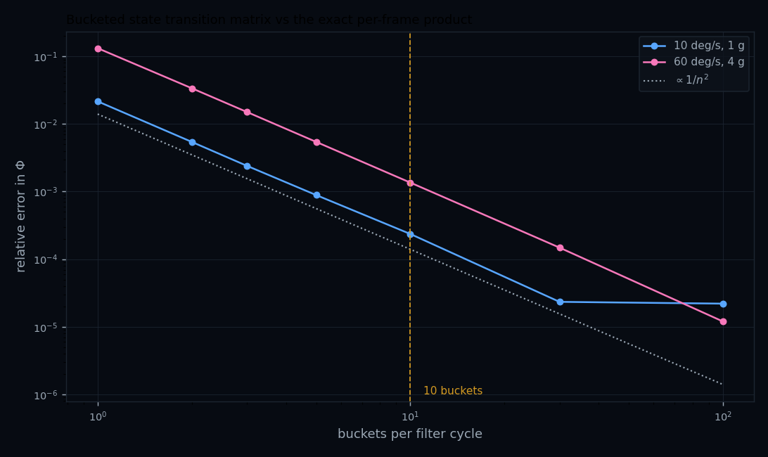
ekf_two_rate.py. Both cases track the $1/n^2$ reference over the
useful range; the benign curve flattens past 30 buckets for the reason given below.
At 60 °/s and 4 g the 10-bucket error is $1.36\times10^{-3}$ — about six times worse than the benign case, which is the expected behaviour: the harder the manoeuvre, the more $F$ moves within a bucket. Note also that the aggressive case has not hit the ripple floor by 100 buckets, because its genuine variation still dominates the quantization term there. Bucket count is a dynamics-dependent tuning parameter, not a universal constant.
Step 4 — propagate, then update
One time update for the whole 300-frame span:
$$ \delta\mathbf x^-_m = \Phi_m\,\delta\mathbf x^+_{m-1} = \mathbf 0, \qquad P^-_m = \Phi_m P^+_{m-1} \Phi_m^{\mathsf T} + Q_m $$The error state propagates to zero because the previous cycle's correction was already handed to the mechanization and the error state reset — the filter estimates the error remaining, and only $P$ carries memory across cycles. The process noise for the interval is
$$ Q_m = \int_0^{\Delta T}\! \Phi(\xi) G W G^{\mathsf T} \Phi(\xi)^{\mathsf T} d\xi \;\approx\; \operatorname{diag}\big( \sigma^2_{\text{VRW}},\, \sigma^2_{\text{ARW}},\, \tfrac{2\sigma^2_{b_a}}{\tau_a},\, \tfrac{2\sigma^2_{b_g}}{\tau_g}\big)\,\Delta T $$then each measurement is applied as an independent scalar update, in a fixed order:
$$ \text{for each scalar } i: \quad K_i = \frac{P\,\mathbf h_i^{\mathsf T}}{\mathbf h_i P \mathbf h_i^{\mathsf T} + R_i}, \qquad \delta\mathbf x \mathrel{+}= K_i\big(z_i - \mathbf h_i \delta\mathbf x\big), \qquad P \leftarrow (I - K_i \mathbf h_i) P $$Step 5 — hand the correction back
$$ \mathbf c_m = -\,\delta\hat{\mathbf x}^+_m, \qquad t(\mathbf c_m) = t_m $$The mechanization applies the position, velocity and attitude parts at the buffered state for epoch $t_m$ and then re-integrates forward to the present, because by the time the filter finished, the fast loop has already run on past it. The bias and scale-factor parts go into the compensation of Step 1 for all subsequent frames, which is what closes the loop: a better bias estimate makes the next 300 increments cleaner, which makes the next $\bar F$ more accurate.
Two asymmetries are worth noticing in that listing. The fast loop does no covariance arithmetic — no 15×15 matrix is touched 300 times a second. And the filter does no integration: it never sees a $\Delta V$ or a $\Delta\theta$, only the accumulated $F$ sums they produced and the buffered states they generated. That division is what makes a navigation-grade filter affordable on flight hardware.
Running it: a verified implementation
Everything above is implemented and checked in a single self-contained script. It synthesises IMU outputs with the three-rate structure of §increments — 1800 Hz sub-samples, two 600 Hz angle increments, one 300 Hz $\Delta V$ shifted back by three sub-samples — applies the documented error model per sub-sample, and runs the two-rate filter exactly as §one full EKF cycle describes.
What it generates
The truth trajectory is defined by a body-rate and specific-force profile and then integrated, so the ideal increments are exact integrals of that profile rather than finite differences of a sampled path. On top of the ideal increments, per sub-sample, in this order:
| Term | Form | Applied to |
|---|---|---|
| FOGM bias | $x_k = (1-\beta\,dt)\,x_{k-1} + \sqrt{2\sigma^2\beta}\;n\sqrt{dt}$ | both, as $x_k\,dt$ |
| Turn-on bias | drawn once per power cycle | both, as $b_0\,dt$ |
| Scale factor | static + FOGM, multiplies the increment | both — generated, never estimated |
| Misalignment / non-orthogonality | off-diagonal $M$, multiplies the increment | both |
| Random walk | $\sigma_{\text{rw}}\,n\sqrt{dt}$ (VRW, ARW) | both |
| Quantization | $\lfloor \cdot/q \rfloor q$ with residual carry | both; gyro dither added before the floor, excluded from the carry |
| Anti-alias filter | symmetric 12-tap over previous + current sub-samples | $\Delta V$ only — never the angle increments |
Error magnitudes are representative navigation-grade figures (0.0035 °/hr gyro bias, 25 µg accelerometer bias, 5 ppm and 100 ppm scale factor) of the right order for the grade rather than any particular part's specification. The quantization steps are round illustrative LSBs for the same reason.
How it verifies itself
A simulation that merely runs proves nothing, so each claim is a check that can fail. The most useful of them is the error-free reproduction test: with every error source, the quantizer and the anti-alias filter disabled, a perfect sensor must reproduce the truth trajectory. It is run before any other result is reported, and it earned its place — it caught two real bugs in the half-frame bookkeeping during development (see the callout below).
| Check | What would fail it | Measured |
|---|---|---|
| Anti-alias centroid | a $\Delta V$ epoch that is not the frame boundary | $t_k + 0.0000$ ms; taps sum to exactly 6 |
| Zero-rotation control | an error in the translation integration | 6.5 × 10⁻¹² m |
| Algorithm faithfulness | cache, epoch or midpoint-rotation mistakes | 0.000 × 100 (bit-identical) |
| vs 1800 Hz truth | — irreducible, see below | 5.3 µm, 2.4 µm/s, 1.8 × 10⁻¹⁵ rad |
| Midpoint rule | rotating $\Delta V$ by the wrong attitude | 4.1 × 10⁻⁷ m/s, vs 8.6 mm/s at the frame start |
| Φ bucketing | a bucket count too low for the dynamics | slope 2.00; 2.4 × 10⁻⁴ at 10 buckets |
| Filter consistency | an optimistic covariance | NIS 1.017 over 420 updates, interval [0.865, 1.135] |
Results
A 120 s run at 300 Hz — 36,000 mechanized frames from 216,000 synthesised sub-samples, with a 1 Hz GNSS position fix — settles to the following steady-state RMS errors over the second half:
| Quantity | Steady-state RMS | Note |
|---|---|---|
| Position | 2.07 m | against a 1.5 m per-axis fix |
| Velocity | 0.054 m/s | never measured directly |
| Tilt | 146 µrad | observable through the specific force |
| Heading | 64 µrad | observable only while manoeuvring |
| Accelerometer bias | 25.4 µg | weakly observable in the vertical |
| Gyro bias | 0.0046 °/hr | comparable to the turn-on spec |
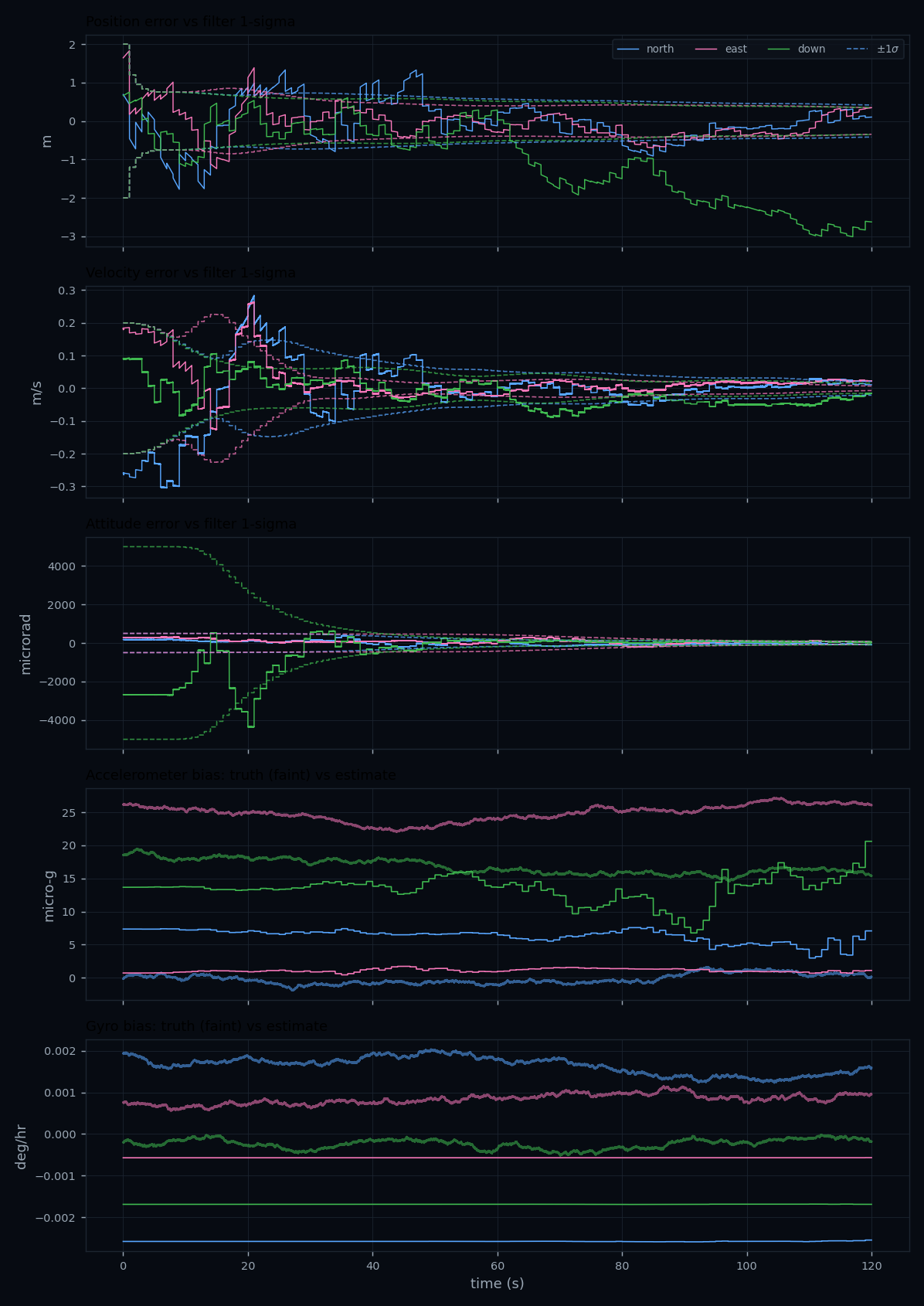
One plotting bug worth naming, because it is easy to ship: the first version drew a single $\sigma$ band for all three axes of each group. Heading $\sigma$ is an order of magnitude larger than tilt $\sigma$, so that made the heading channel look divergent when it was not. Each axis now carries its own envelope.
The time-of-validity experiment
The script runs the same measurements through two otherwise identical filters: one forms the residual against the buffered state at the fix epoch, the other against the latest state. With the fix valid 0.37 s before the filter boundary:
| Run length | Residual vs buffered state | Residual vs latest state | Ratio |
|---|---|---|---|
| 12 s | 1.50 m | 5.98 m | 4.0× |
| 30 s | 0.86 m | 88.5 m | 103× |
| 60 s | 0.74 m | 268 m | 360× |
| 120 s | 2.08 m | 642 m | 309× |
Filter consistency, and what the 15-state vector leaves out
Scale factor, misalignment and non-orthogonality are generated but never estimated — a realistic choice, and one whose cost is measured rather than hidden. Normalised innovation squared (NIS) should average 1 for a consistent filter; over 60 s runs:
| Configuration | Mean NIS | Verdict |
|---|---|---|
| As shipped, all error terms active | 1.017 | consistent |
| Scale factor removed from the sensor | 1.010 | consistent |
| Perfect sensor | 0.999 | consistent |
So un-modelled sensor error accounts for about +0.019 of the excess and scale factor alone for +0.008. A real filter closes that gap either by putting scale factor in the state vector or by inflating $Q$ deliberately to cover it.
Coning and sculling — and who is responsible for them
These two effects come from the same fact: rotations do not commute, and over a finite interval the attitude is changing while you integrate.
Coning
If two body axes oscillate with a phase difference, the body traces a cone and accumulates a real, secular rotation about the third axis. Naively summing the angle increments as if they were vectors misses it entirely, because vector addition is commutative and rotation is not. The first-order correction restores the missing term:
$$ \Delta\boldsymbol\theta^{\text{corrected}} = \Delta\boldsymbol\theta_a + \Delta\boldsymbol\theta_b + \underbrace{\tfrac{1}{2}\,\Delta\boldsymbol\theta_a \times \Delta\boldsymbol\theta_b}_{\text{coning}}. $$The cross product of the two half-increments recovers part of what a single full-frame sum throws away. It is worth being careful about what that does and does not explain — see the callout immediately below. For a sinusoidal two-axis oscillation of amplitude $A$ at angular frequency $\omega$, in quadrature, the drift rate of the uncorrected sum is
$$ \dot\theta_{\text{coning}} \approx \tfrac{1}{2} A^2 \omega . $$That quadratic dependence on amplitude is brutal. Evaluated numerically at 5 Hz:
| Amplitude | Closed form $A^2\omega/2$ | Numeric |
|---|---|---|
| 1° | 0.274 °/s | 0.274 °/s |
| 3° | 2.47 °/s | 2.46 °/s |
| 6° | 9.87 °/s | 9.79 °/s |
Tripling the amplitude multiplies the drift by nine. A 6° quadrature oscillation at 5 Hz — well within what airframe flex or a vibrating mount can produce — makes an uncorrected attitude solution useless within seconds.
Sculling
The velocity analogue. If the body rotates while it accelerates, and the two oscillate in phase, the product rectifies into a steady velocity error. The correction has the same shape:
$$ \Delta\mathbf v^{\text{corrected}} = \Delta\mathbf v + \underbrace{\tfrac{1}{2}\,\Delta\boldsymbol\theta \times \Delta\mathbf v}_{\text{rotation}} + \underbrace{\tfrac{1}{2}\big(\Delta\boldsymbol\theta_a \times \Delta\mathbf v_b + \Delta\mathbf v_a \times \Delta\boldsymbol\theta_b\big)}_{\text{sculling}} . $$Measured for a 2° oscillation against 5 m/s² in phase at 5 Hz, comparing a fine integration against what a consumer can reconstruct from block sums alone:
| Output interval | Velocity error rate | Over 10 s |
|---|---|---|
| 3.33 ms (300 Hz) | 0.08 mm/s per s | 0.8 mm/s |
| 10 ms (100 Hz) | 0.72 mm/s per s | 7.2 mm/s |
| 20 ms (50 Hz) | 2.8 mm/s per s | 28 mm/s |
The error scales roughly as $\Delta t^2$, which is the practical argument for a high output rate: going from 50 Hz to 300 Hz cuts the uncorrected sculling error by a factor of ~35.
Where the correction actually happens
This is the part most often got wrong, and it is a hardware question rather than a software one.
| Effect | Needs | Who can do it |
|---|---|---|
| Coning | Sub-interval angular history | Inside the IMU. Only the unit sees its own internal samples |
| Sculling | Sub-interval angular and linear history | Inside the IMU, same reason |
| Velocity-frame rotation | Attitude at the increment's midpoint | Navigation software — it owns the attitude |
| Window alignment | Knowing each output's time of validity | Navigation software — and it must cache across frames |
A lower-grade unit that reports only sampled rate and acceleration shifts the burden the other way: with no sub-interval information published at all, the consumer has to sample fast enough that coning and sculling are negligible, which is usually not achievable. That is the real reason increment output is worth paying for.
Integration details that cost you accuracy
- Time-tagging. If the IMU's sample epoch is uncertain by $\delta t$ while rotating at $\omega$, you inject an attitude error $\omega\,\delta t$ — at 100 °/s a 1 ms uncertainty is 0.1°, larger than everything else in the budget. Use the hardware sync/PPS pin, not the arrival time of the packet.
- Which window, not just which instant. Per time of validity above, each output has its own interval and $\Delta\mathbf v$ typically lags the angle increments. Align them before mechanizing, and cache across the frame boundary if the unit publishes a split $\Delta\boldsymbol\theta$.
- Rate vs increment output. Prefer $\Delta\theta/\Delta v$ (integrated increments) over sampled rate: increments are inherently coning/sculling-friendly and immune to sample-time jitter.
- Mounting and thermal path. The lever arm from IMU to the GNSS antenna must be measured to the millimetre; thermal gradients across the block show up directly as bias.
- Vibration. Check the vibration-rectification-error spec, not just the noise floor — MEMS can turn a symmetric vibration into a DC acceleration bias.
Planned bench work
- Multi-hour static logs → Allan-variance curves per axis, compared to the datasheet.
- Turn-on repeatability over dozens of power cycles and a temperature sweep.
- Free-inertial drift race between grades on the same trajectory.
- Gyrocompassing convergence time vs latitude and averaging window.
Related: IMU theory & error model · gyroscope technologies · alt-PNT · back to Hardware.